Tutorial – Comparing means under controlled conditions
Diplôme Universitaire en Bioinformatique Intégrative (DUBii)
Jacques van Helden
2020-03-12
Introduction
This tutorial aims at providing an empirical introduction to the application of mean comparison tests to omics data.
The goals include
- revisiting the basic underlying concepts (sampling, estimation, hypothesis testing, risks…);
- perceiving the problems that arise when a test of hypothesis is applied on several thousand of features (multiple testing);
- introducing some methods to circumvent these problems (multiple testing corrections);
using graphical representations in order to grasp the results of several thousand tests in a winkle of an eye:
- p-value histogram
- MA plot
- volcano plot
The whole tutorial will rely on artificial data generated by drawing random numbers that follow a given distribution of probabilities (in this case, the normal distribution, but other choices could be made afterwards).
The tutorial will proceed progressively:
Generate a multivariate table (with individuals in columns and features in rows) and fill it with random data following a given distribution of probability.
Measure different descriptive parameters on the sampled data.
Use different graphical representations to visualise the data distribution.
Run a test of hypothesis on a given feature.
Run the same test of hypothesis on all the features.
Use different graphical representations to summarize the results of all the tests.
Apply different corrections for multiple testing (Bonferroni, Benjamini-Hochberg, Storey-Tibshirani q-value).
Compare the performances of the test depending on the chosen multiple testing correction.
Experimental setting
Well, by “experimental” we mean here that we will perform in silico experiments.
Let us define the parameters of our analysis. We will generate data tables of artificial data following normal distributions, with either different means (tests under \(H_1\)) or equal means (tests under \(H_0\)).
We will do this for a number of features \(m_0=10,000\) (number of rows in the “\(H_0\)” data table), which could be considered as replicates to study the impact of sampling fluctuations.
In a second time (not seen here) we could refine the script by running a sampling with a different mean for each feature, in order to mimic the behaviour of omics datasets (where genes have different levels of expression, proteins and metabolite different concentrations).
Parameters
| Parameter | Value | Description |
|---|---|---|
| \(n_1\) | \({2, 3, 4, 8, 16, 32, 64}\) | size of the sample from the first population. individual choice. Each participant will choose a given sample size |
| \(n_2\) | \(= n_1\) | size of the sample from the second population |
| \(\mu_1\) | 10 or 7 | mean of the first population. each participant will chose one value |
| \(\mu_2\) | 10 | mean of the second population |
| \(\sigma_1\) | 2 | Standard deviation of the first population |
| \(\sigma_2\) | 3 | Standard deviation of the second population |
| \(m_0\)$ | \(10,000\) | number of features under null hypothesis |
Sample sizes
Each participant will choose a different sample size among the following values: \(n \in {2, 3, 4, 5, 8, 16, 64}\). Noteowrthy, many omics studies are led with a very small number of replicates (frequently 3), so that it will be relevant to evaluate thee impact of the statistical sample size (number of replicates) on the sensibility (proportion of cases declared positive under \(H_1\)).
Performances of the tests
We will measure the performances of a test by running \(r = 10,000\) times under \(H_0\), and \(r = 10,000\) times under \(H_1\).
- count the number of \(FP\), \(TP\), \(FN\), \(TN\)
- compute the derived statistics: \(FPR\), \(FDR\) and \(Sn\)
\[FPR = \frac{FP}{m_0} = \frac{FP}{FP + TN} \]
\[FDR = \frac{FP}{\text{Positive}} = \frac{FP}{FP + TP} \]
\[Sn = \frac{TP}{m_1} = \frac{TP}{TP + FN} \] \[PPV = \frac{TP}{\text{Positive}} = \frac{TP}{TP + FP}\]
Recommendations
Coding recommendations
Choose a consistent coding style, consistent with a reference style guide (e.g. Google R Syle Guide). In particular:
- For variable names, use the camel back notation with a leading lowercase (e.g.
myDataTable) rather than the dot separator (my.data.table) - For variable names, use the camel back notation with a leading uppercase (e.g.
MyMeanCompaTest).
- For variable names, use the camel back notation with a leading lowercase (e.g.
Define your variables with explicit names (sigma, mu rather than a, b, c, …).
Comment your code
- indicate what each variable represents
- before each segment of code, explain what it will do
Ensure consistency between the code and the report \(\rightarrow\) inject the actual values of the R variables in the markdown.
Scientific recommendations
Explicitly formulate the statistical hypotheses before running a test.
Discuss the assumptions underlying the test: are they all fulfilled? If not explain why (e.g. because we want to test the impact of this parameter, …) .
Tutorial
Part 1: generating random datasets
Define your parameters
Write a block of code to define the parameters specified aboce.
Note that each participant will have a different value for the sample sizes (\(n_1, n_2\)).
#### Defining the parameters ####

## Sample sizes.
## This parameter should be defined individually for each participant
n1 <- 16 # sample size for the first group
n2 <- 16 # ssample size for second group

## First data table
m <- 1000 # Number of features
mu1 <- 7 # mean of the first population
mu2 <- 10 # mean of the second population

## Standard deviations
sigma1 <- 2 # standard deviation of the first population
sigma2 <- 3 # standard deviation of the second population

## Significance threshold.
## Note: will be applied successively on the different p-values
## (nominal, corrected) to evaluate the impact
alpha <- 0.05
The table below lists the actual values for my parameters (your values for \(n_i\) will be different).
| Parameter | Value | Description |
|---|---|---|
| \(\mu_1\) | 7 | Mean of the first population |
| \(\mu_2\) | 10 | Mean of the second population |
| \(\sigma_1\) | 2 | Standard deviation of the first population |
| \(\sigma_2\) | 2 | Standard deviation of the second population |
| \(n_1\) | 16 | Sample size for the first group |
| \(n_2\) | 16 | Sample size for the second group |
Generate random data sets
Exercise:
Generate an data frame named
group1which with \(m_0\) rows (the number of features under \(H_0\), defined above) and \(n_1\) columns (sample size for the first population), filled with random numbers drawn from the first population.Name the columns with labels indicating the group and sample number:
g1s1, ,g1s2… with indices from 1 \(n_1\).Name the rows to denote the feature numbers:
ft1,ft2, … with indices from 1 to \(m_0\).Check the dimensions of
group1.Print its first and last rows to check its content and the row and column names.
Generate a second data frame named
group2for the samples drawn from the second population with the appropriate size, and name the columns and rows consistently.
Useful functions
rnorm()matrix()data.frame()paste()paste0()colnames()rownames()dim()
Trick:
- the funciton
matrix()enables us to define the number of columns and the number of rows, - the function
data.frames()does not enable this, but it can take as input a matrix, from which it will inherit the dimensions
Solution (click on the “code” button to check the solution).
#### Generate two tables (one per population) with the random samples ####

## Info: for didactiv purpose we will use a progressive approach to generate
## the data the first group,  and a more compact formulation (in one command)
## for the second group.

## Dataset under H0, with a progressive approach

## Generate a vector of size m*n1 with all the random values
## for each feature and each infividual
normVector <- rnorm(n = m * n1, mean = mu1, sd = sigma1)

## Wrap the vector in an m x n1 matrix
normMatrix <- matrix(data = normVector,
                     nrow = m,
                     ncol = n1)

## Create a data frame with the content of this matrix
group1 <- data.frame(normMatrix)

## Set the column and row names
colnames(group1) <- paste(sep = "", "g1s", 1:n1)
rownames(group1) <- paste(sep = "", "ft", 1:m)

## Dataset under H1: use a more direct approach, compact the 3 steps in a single command
group2 <- data.frame(
  matrix(data = rnorm(n = m * n2, mean = mu2, sd = sigma2),
         nrow = m,
         ncol = n2))
colnames(group2) <- paste(sep = "", "g2s", 1:n2)
rownames(group2) <- paste(sep = "", "ft", 1:m)
Check the content of the data table from the first group.
[1] 1000 16| g1s1 | g1s2 | g1s3 | g1s4 | g1s5 | g1s6 | g1s7 | g1s8 | g1s9 | g1s10 | g1s11 | g1s12 | g1s13 | g1s14 | g1s15 | g1s16 | |
|---|---|---|---|---|---|---|---|---|---|---|---|---|---|---|---|---|
| ft1 | 8.941285 | 6.065904 | 6.865641 | 4.859670 | 4.512642 | 6.895100 | 6.958049 | 6.571121 | 6.346707 | 9.316831 | 2.405495 | 7.560588 | 5.237921 | 7.455899 | 9.150481 | 7.584783 |
| ft2 | 6.341780 | 5.572643 | 6.225146 | 7.607175 | 7.916639 | 9.159623 | 5.848137 | 3.714532 | 5.690572 | 8.518993 | 7.721817 | 8.796947 | 8.394252 | 5.201240 | 5.078987 | 5.059495 |
| ft3 | 7.256030 | 5.609690 | 5.085780 | 6.251178 | 6.185095 | 5.746095 | 5.426706 | 5.937105 | 3.509892 | 9.136032 | 6.853375 | 6.274303 | 7.318755 | 4.817723 | 10.016098 | 8.024319 |
| ft4 | 7.306063 | 9.761042 | 6.510410 | 2.995976 | 7.084978 | 9.170946 | 5.843874 | 7.777505 | 6.699460 | 7.871503 | 4.288901 | 11.089438 | 7.985812 | 6.003219 | 2.376816 | 7.505029 |
| ft5 | 7.377395 | 5.728367 | 7.502510 | 6.681304 | 5.280177 | 4.125594 | 10.377625 | 2.956254 | 4.353912 | 8.138003 | 9.110175 | 8.887401 | 8.325482 | 5.321332 | 6.616982 | 4.688656 |
| ft6 | 8.138350 | 7.867051 | 7.211847 | 9.442536 | 3.512614 | 7.266573 | 5.658330 | 7.845747 | 9.028672 | 7.819257 | 10.218765 | 4.371628 | 6.856506 | 6.572069 | 4.021843 | 5.959517 |
| g1s1 | g1s2 | g1s3 | g1s4 | g1s5 | g1s6 | g1s7 | g1s8 | g1s9 | g1s10 | g1s11 | g1s12 | g1s13 | g1s14 | g1s15 | g1s16 | |
|---|---|---|---|---|---|---|---|---|---|---|---|---|---|---|---|---|
| ft995 | 9.605869 | 5.740994 | 7.952485 | 6.786263 | 8.301584 | 5.963019 | 8.111063 | 3.566636 | 8.257055 | 6.686423 | 9.280676 | 9.945114 | 7.836719 | 5.139963 | 6.322468 | 3.879234 |
| ft996 | 8.049430 | 8.322572 | 9.308645 | 6.249635 | 6.517046 | 6.945753 | 10.476903 | 8.258785 | 9.631009 | 5.271014 | 8.183092 | 4.636647 | 7.828096 | 4.856097 | 7.808470 | 4.576391 |
| ft997 | 7.713957 | 8.750733 | 9.170241 | 6.859514 | 5.216096 | 8.194377 | 8.951150 | 7.481994 | 6.736394 | 5.140652 | 10.301499 | 5.520028 | 8.206613 | 4.289319 | 6.971314 | 8.807768 |
| ft998 | 9.826277 | 5.728074 | 7.169590 | 9.398133 | 6.224335 | 6.586678 | 10.960816 | 4.886410 | 9.327067 | 10.245310 | 5.790441 | 3.356992 | 7.388533 | 6.234348 | 6.130373 | 4.776949 |
| ft999 | 10.307381 | 8.634587 | 7.994570 | 8.684634 | 3.655567 | 7.106540 | 5.869480 | 5.938656 | 8.157128 | 7.209484 | 5.526127 | 2.734005 | 6.518238 | 8.962575 | 6.742045 | 7.910900 |
| ft1000 | 6.695509 | 8.701822 | 10.610700 | 9.227807 | 5.761689 | 9.165080 | 6.451053 | 6.774868 | 7.586023 | 10.825243 | 6.221651 | 7.521273 | 6.485664 | 6.469598 | 3.654353 | 7.192678 |
Check the content of the data table from the second group.
[1] 1000 16| g2s1 | g2s2 | g2s3 | g2s4 | g2s5 | g2s6 | g2s7 | g2s8 | g2s9 | g2s10 | g2s11 | g2s12 | g2s13 | g2s14 | g2s15 | g2s16 | |
|---|---|---|---|---|---|---|---|---|---|---|---|---|---|---|---|---|
| ft1 | 10.222202 | 6.803465 | 5.644039 | 15.310530 | 12.022135 | 9.205384 | 7.810089 | 6.824159 | 9.601778 | 3.042279 | 13.646228 | 12.040121 | 13.800577 | 5.405056 | 11.868858 | 5.146461 |
| ft2 | 13.788490 | 11.414270 | 19.247855 | 9.104344 | 7.161907 | 14.430186 | 6.693538 | 11.771966 | 5.466395 | 13.846364 | 4.814672 | 10.611065 | 14.007772 | 9.264401 | 11.794563 | 11.574728 |
| ft3 | 8.218564 | 9.340666 | 11.842295 | 13.045543 | 5.242310 | 7.199965 | 12.454361 | 11.112718 | 9.344606 | 11.487924 | 10.799383 | 4.877696 | 6.419245 | 13.373079 | 13.581551 | 10.329964 |
| ft4 | 6.388767 | 14.841495 | 6.673942 | 6.147528 | 7.040335 | 15.048979 | 7.286110 | 7.894366 | 13.823895 | 14.894529 | 8.177395 | 11.067993 | 12.745004 | 13.283611 | 8.662708 | 6.765320 |
| ft5 | 7.862331 | 8.373275 | 4.457363 | 11.435550 | 12.882556 | 13.882535 | 5.722801 | 12.662282 | 3.671602 | 17.983611 | 4.309335 | 10.602149 | 7.648618 | 8.398105 | 11.239692 | 8.139710 |
| ft6 | 15.439498 | 5.644524 | 9.878748 | 5.295041 | 4.737427 | 11.884359 | 7.842318 | 15.196238 | 10.719587 | 12.656550 | 7.791976 | 8.960966 | 11.817566 | 4.536809 | 8.054717 | 6.694868 |
| g2s1 | g2s2 | g2s3 | g2s4 | g2s5 | g2s6 | g2s7 | g2s8 | g2s9 | g2s10 | g2s11 | g2s12 | g2s13 | g2s14 | g2s15 | g2s16 | |
|---|---|---|---|---|---|---|---|---|---|---|---|---|---|---|---|---|
| ft995 | 11.560118 | 11.477506 | 7.288923 | 7.257060 | 7.974623 | 11.264721 | 10.600428 | 10.025548 | 7.492476 | 15.06344 | 8.820455 | 15.313801 | 9.524212 | 8.412263 | 14.001309 | 9.712662 |
| ft996 | 6.675313 | 12.578788 | 9.168974 | 8.874279 | 12.924633 | 8.100163 | 9.838190 | 9.654799 | 8.691387 | 12.08811 | 8.808767 | 10.163288 | 10.591247 | 11.112719 | 7.381530 | 4.043808 |
| ft997 | 9.429636 | 10.788576 | 7.365419 | 6.562660 | 12.170922 | 11.668521 | 9.720355 | 14.542886 | 9.716674 | 11.50710 | 12.884846 | 7.063525 | 4.797859 | 8.954747 | 5.540972 | 9.692725 |
| ft998 | 8.826315 | 11.819484 | 5.649444 | 10.404189 | 14.148555 | 8.348604 | 4.936733 | 14.004160 | 4.741586 | 10.12474 | 8.560174 | 7.037552 | 6.882366 | 9.336428 | 6.524944 | 7.723506 |
| ft999 | 14.302763 | 5.136343 | 5.557525 | 4.767551 | 12.962332 | 8.779562 | 9.618915 | 15.235528 | 13.498886 | 10.64103 | 10.652171 | 10.128990 | 8.093268 | 6.784517 | 7.035637 | 9.486925 |
| ft1000 | 7.111972 | 15.204233 | 13.274704 | 13.993838 | 7.358308 | 14.302453 | 7.925037 | 9.124976 | 12.256743 | 12.69099 | 7.320802 | 10.944899 | 12.102726 | 8.468052 | 7.981384 | 6.673717 |
Checking the properties of the data tables
Check the properties of the columns (individuals, e.g. biological samples) and rows (features, e.g. genes or proteins or metabolites) of the data tables.
Use the
summary()funciton to quickly inspect the column-wise properties (statistics per individual).Use
apply(),mean()andsd()to generate a data frame that collects- the column-wise parameters (statistics per feature)
- the row-wise parameters (statistics per feature).
      g1s1             g1s2              g1s3              g1s4              g1s5              g1s6             g1s7              g1s8              g1s9            g1s10             g1s11            g1s12            g1s13             g1s14            g1s15            g1s16
 Min.   : 1.153   Min.   : 0.2647   Min.   :-0.8534   Min.   : 0.9221   Min.   : 0.2519   Min.   : 1.098   Min.   :-0.6261   Min.   : 0.5412   Min.   :-2.541   Min.   : 0.4808   Min.   : 1.537   Min.   : 0.614   Min.   : 0.3706   Min.   :-0.904   Min.   : 1.078   Min.   : 0.2331
 1st Qu.: 5.574   1st Qu.: 5.7378   1st Qu.: 5.6475   1st Qu.: 5.7334   1st Qu.: 5.7508   1st Qu.: 5.718   1st Qu.: 5.5893   1st Qu.: 5.5918   1st Qu.: 5.565   1st Qu.: 5.6125   1st Qu.: 5.567   1st Qu.: 5.431   1st Qu.: 5.5188   1st Qu.: 5.503   1st Qu.: 5.699   1st Qu.: 5.7006
 Median : 6.868   Median : 7.2550   Median : 7.0104   Median : 7.0928   Median : 7.1135   Median : 7.106   Median : 6.9690   Median : 6.9331   Median : 6.979   Median : 7.1559   Median : 7.057   Median : 6.877   Median : 6.9950   Median : 6.899   Median : 6.987   Median : 7.0582
 Mean   : 6.891   Mean   : 7.1632   Mean   : 6.9962   Mean   : 7.1103   Mean   : 7.0383   Mean   : 7.107   Mean   : 6.9354   Mean   : 6.9583   Mean   : 6.987   Mean   : 7.0500   Mean   : 7.049   Mean   : 6.846   Mean   : 6.9139   Mean   : 6.959   Mean   : 7.005   Mean   : 6.9945
 3rd Qu.: 8.174   3rd Qu.: 8.5433   3rd Qu.: 8.3104   3rd Qu.: 8.4067   3rd Qu.: 8.2805   3rd Qu.: 8.506   3rd Qu.: 8.2376   3rd Qu.: 8.2567   3rd Qu.: 8.349   3rd Qu.: 8.4553   3rd Qu.: 8.461   3rd Qu.: 8.207   3rd Qu.: 8.3111   3rd Qu.: 8.348   3rd Qu.: 8.262   3rd Qu.: 8.3510
Max. :14.239 Max. :12.3955 Max. :13.7764 Max. :14.7685 Max. :15.2060 Max. :13.430 Max. :13.3995 Max. :13.1033 Max. :14.015 Max. :13.6878 Max. :13.513 Max. :13.384 Max. :12.5050 Max. :13.272 Max. :13.596 Max. :12.9327 g2s1 g2s2 g2s3 g2s4 g2s5 g2s6 g2s7 g2s8 g2s9 g2s10 g2s11 g2s12 g2s13 g2s14 g2s15 g2s16
Min. : 0.4878 Min. :-1.210 Min. : 2.164 Min. :-0.07996 Min. : 0.2839 Min. : 0.05548 Min. : 0.4454 Min. : 0.598 Min. : 1.132 Min. : 0.1758 Min. :-1.166 Min. : 1.895 Min. :-0.6536 Min. : 1.289 Min. :-0.7888 Min. :-0.0963
1st Qu.: 7.8010 1st Qu.: 8.025 1st Qu.: 7.959 1st Qu.: 8.07439 1st Qu.: 7.8946 1st Qu.: 8.02792 1st Qu.: 8.0490 1st Qu.: 7.798 1st Qu.: 8.122 1st Qu.: 8.0893 1st Qu.: 8.050 1st Qu.: 8.090 1st Qu.: 7.8425 1st Qu.: 8.126 1st Qu.: 7.9821 1st Qu.: 8.0623
Median :10.0579 Median : 9.916 Median :10.021 Median : 9.92345 Median :10.0376 Median : 9.99913 Median :10.0563 Median :10.013 Median :10.071 Median :10.0239 Median : 9.844 Median :10.022 Median : 9.9218 Median :10.060 Median : 9.8194 Median :10.0806
Mean : 9.8699 Mean : 9.985 Mean : 9.965 Mean :10.00777 Mean :10.0254 Mean :10.05125 Mean :10.0442 Mean : 9.945 Mean :10.129 Mean :10.0470 Mean : 9.965 Mean :10.104 Mean : 9.9233 Mean : 9.961 Mean : 9.9155 Mean :10.0670
3rd Qu.:11.7515 3rd Qu.:11.961 3rd Qu.:11.942 3rd Qu.:12.03088 3rd Qu.:12.0975 3rd Qu.:12.10682 3rd Qu.:12.0168 3rd Qu.:11.963 3rd Qu.:12.214 3rd Qu.:12.0801 3rd Qu.:12.018 3rd Qu.:12.244 3rd Qu.:12.0490 3rd Qu.:12.005 3rd Qu.:11.9846 3rd Qu.:12.0891
Max. :19.6257 Max. :19.358 Max. :20.257 Max. :20.79365 Max. :20.4195 Max. :20.66677 Max. :19.9660 Max. :18.719 Max. :19.274 Max. :20.0369 Max. :19.276 Max. :19.836 Max. :20.0104 Max. :19.669 Max. :18.6784 Max. :20.0330 ## Columns-wise statistics
colStats <- data.frame(
m1 = apply(group1, MARGIN = 2, mean),
m2 = apply(group2, MARGIN = 2, mean),
s1 = apply(group1, MARGIN = 2, sd),
s2 = apply(group2, MARGIN = 2, sd)
)
## Row-wise statistics
rowStats <- data.frame(
m1 = apply(group1, MARGIN = 1, mean),
m2 = apply(group2, MARGIN = 1, mean),
s1 = apply(group1, MARGIN = 1, sd),
s2 = apply(group2, MARGIN = 1, sd)
)Add a column with the difference between sample means for each feature.
Tips: this can be done in a single operation.
Merge the two groups in a single data frame
In omics data analysis, we typically obtain
- a single data table with all the individuals (biological samples) of all the groups
- a table containing the metadata, i.e. the information about each individual (biological sample)
Two methods could be envisaged a priori:
cbind(), which simply binds the columns of two input tables. This can however be somewhat dangerous, because it assumes that these two tables have the same number of rows (features) and that these rows contain information about the same features in the same order. However, in some cases we dispose of data tables coming from different sources (or software tools), where the features (genes, proteins, metabolites) might have a partial overlap rather than an exact 1-to-1 correspondence, and, even when the feature sets are the same, they might be presented in different orderes.A much safer approach is thus to use
merge(), and to explicitly indicate one or several colummns on which the features from the two table will be unified
In our case, the two data tables only contain numeric data, and the identification will be done on the row names (which contain the feature identifiers ft1, ft2, … that we defined above). In some cases, we will have to merge data table containing different informations, including a column with identifiers (or maybe additional columns e.g. the genotype, conditions, …) and we will use internal columns of the table to unify their rows.
We will create such a structure for further analysis/
## Read the help of the merge() function
# ?merge

## Create a data frame with the merged values
dataTable <- merge(x = group1, y = group2, by = "row.names")
# dim(dataTable) # NOTE: the merged table contains n1 + n2 columns + one additional column Row.names

## Use the Row.names column as names for the merged table
row.names(dataTable) <- dataTable$Row.names
dataTable <- dataTable[, -1] ## Suppress the first column which contained the row names
# dim(dataTable)

## Generate a metadata table
metaData <- data.frame(
  sampleNames = colnames(dataTable),
  sampleGroup = c(rep("g1", length.out = n1), rep("g2", length.out = n2)),
  sampleColor = c(rep("#DDEEFF", length.out = n1), rep("#FFEEDD", length.out = n2))
)

kable(metaData, caption = "Metadata table")| sampleNames | sampleGroup | sampleColor |
|---|---|---|
| g1s1 | g1 | #DDEEFF |
| g1s2 | g1 | #DDEEFF |
| g1s3 | g1 | #DDEEFF |
| g1s4 | g1 | #DDEEFF |
| g1s5 | g1 | #DDEEFF |
| g1s6 | g1 | #DDEEFF |
| g1s7 | g1 | #DDEEFF |
| g1s8 | g1 | #DDEEFF |
| g1s9 | g1 | #DDEEFF |
| g1s10 | g1 | #DDEEFF |
| g1s11 | g1 | #DDEEFF |
| g1s12 | g1 | #DDEEFF |
| g1s13 | g1 | #DDEEFF |
| g1s14 | g1 | #DDEEFF |
| g1s15 | g1 | #DDEEFF |
| g1s16 | g1 | #DDEEFF |
| g2s1 | g2 | #FFEEDD |
| g2s2 | g2 | #FFEEDD |
| g2s3 | g2 | #FFEEDD |
| g2s4 | g2 | #FFEEDD |
| g2s5 | g2 | #FFEEDD |
| g2s6 | g2 | #FFEEDD |
| g2s7 | g2 | #FFEEDD |
| g2s8 | g2 | #FFEEDD |
| g2s9 | g2 | #FFEEDD |
| g2s10 | g2 | #FFEEDD |
| g2s11 | g2 | #FFEEDD |
| g2s12 | g2 | #FFEEDD |
| g2s13 | g2 | #FFEEDD |
| g2s14 | g2 | #FFEEDD |
| g2s15 | g2 | #FFEEDD |
| g2s16 | g2 | #FFEEDD |
Visualisation of the data
Box plot of the sampled values
#### Boxplot of the values per sample ####
boxplot(dataTable,
        col = as.vector(metaData$sampleColor),
        horizontal = TRUE,
        las = 1,
        main = "Sampled values",
        xlab = "X")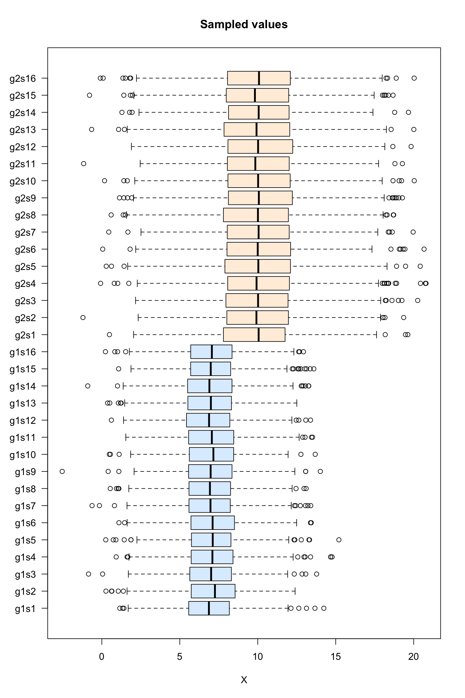
Box plot of the sampled values
Violin plot of the sampled values
#### Boxplot of the values per sample ####
vioplot::vioplot(dataTable,
                 col = as.vector(metaData$sampleColor),
                 horizontal = TRUE,
                 las = 1,
                 main = "Sampled values",
                 xlab = "X")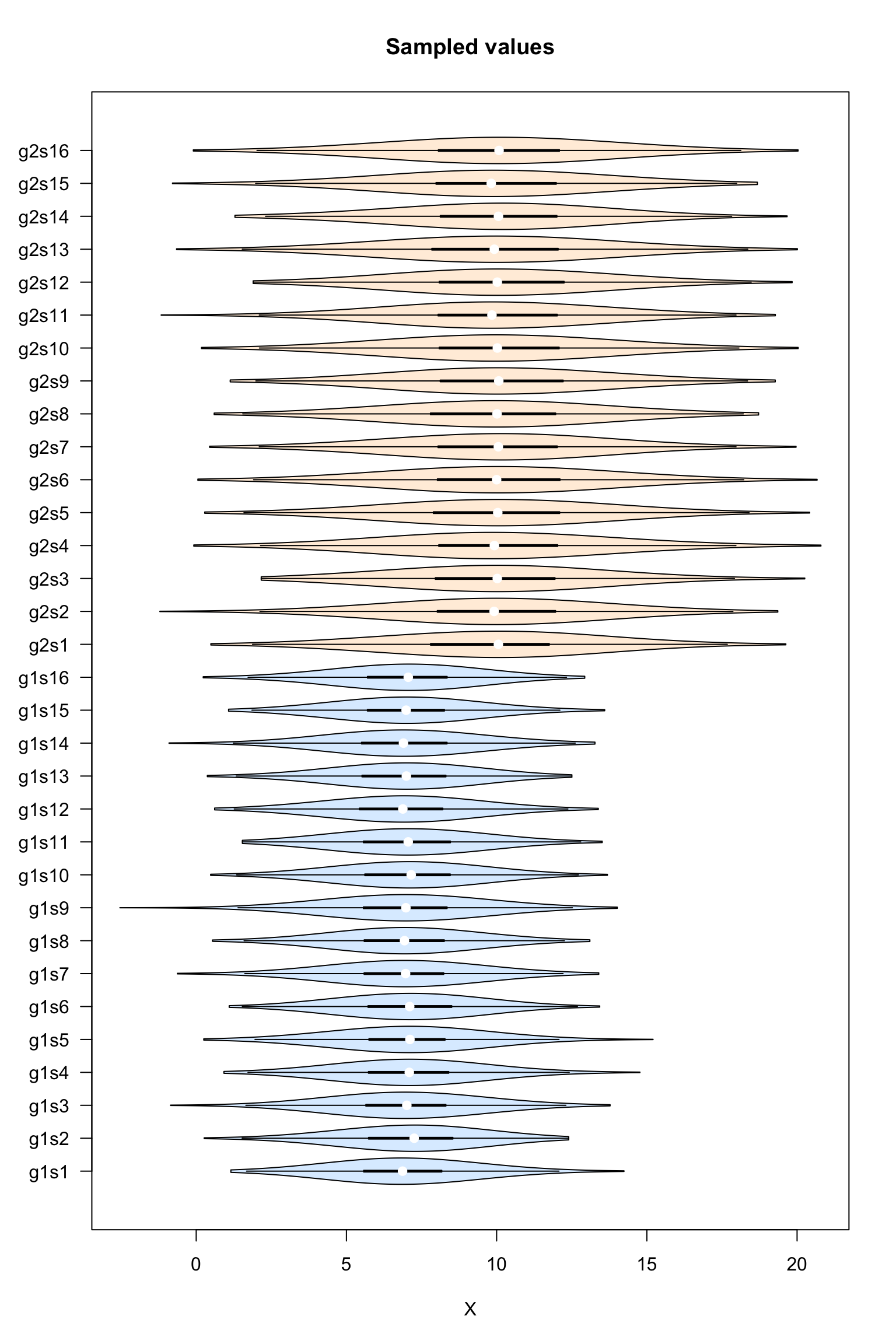
Violin plot of the sampled values
Histogram of the sampled values
- Draw two histograms with all the values group 1 and group2, respectively.
Tip: use mfrow() to display the histogram above each other, and set the limits of the abscissa (x axis) to the same value.
xlim  <- range(append(group1, group2))

## Compute mean and sd for all the samples of group1 and group2, resp
m1 <- mean(unlist(group1))
m2 <- mean(unlist(group2))
s1 <- sd(unlist(group1))
s2 <- sd(unlist(group2))

par(mfrow = c(2,1))
## Plot histogram of Group1 values, and get the values in a variable named h1
h1 <- hist(x = unlist(group1), breaks = 100, col = "#DDEEFF", border = "blue",
     main = "Group 1", xlab = "X", las = 1, xlim = xlim)
abline(v = m1, col = "blue", lwd = 2) ## mark the mean of all samples
arrows(x0 = m1, x1 = m1 + s1,
       y0 = max(h1$counts)/2, y1 = max(h1$counts)/2,
       length = 0.07, angle = 20, col = "blue", lwd = 2, code = 2)
legend("topright",
       legend = c(paste0("m1 = ", round(digits = 2, m1)),
                  paste0("s1 = ", round(digits = 2, s1))))

## Plot histogram of Group2 values, and get the values in a variable named h2
h2 <- hist(x = unlist(group2), breaks = 100, col = "#FFEEDD", border = "brown",
     main = "Group 2", xlab = "X", las = 1, xlim = xlim)
abline(v = mean(unlist(group2)), col = "brown", lwd = 2)
arrows(x0 = m2, x1 = m2 + s2,
       y0 = max(h2$counts)/2, y1 = max(h2$counts)/2,
       length = 0.07, angle = 20, col = "brown", lwd = 2, code = 2)
legend("topright",
       legend = c(paste0("m2 = ", round(digits = 2, m2)),
                  paste0("s2 = ", round(digits = 2, s2))))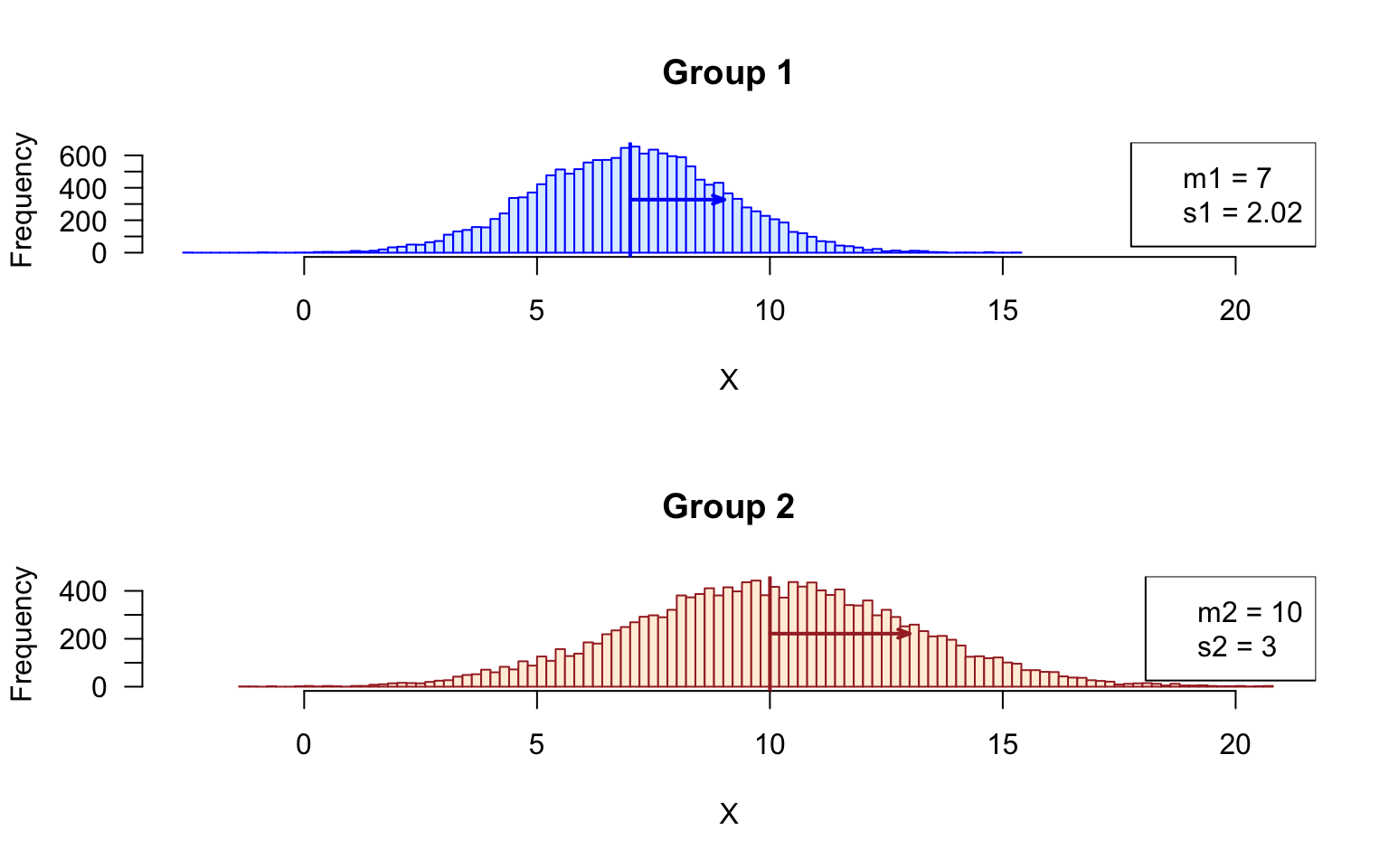
Sampling distribution of the means
Draw histogram with the sampling distribution of the means in the respective groups.
# xlim  <- range(append(colStats$m1, colStats$m2))

## Compute the parameters (mean, sd) of the sampling distributions of the means
mm1 <- mean(rowStats$m1)
mm2 <- mean(rowStats$m2)
se1 <- sd(rowStats$m1)
se2 <- sd(rowStats$m2)

par(mfrow = c(2,1))
## Plot histogram of Group1 values, and get the values in a variable named h1
h1 <- hist(x = rowStats$m1, breaks = 100, col = "#AACCFF", border = "#AACCFF",
     main = "Group 1", xlab = "X", las = 1, xlim = xlim)
abline(v = mm1, col = "blue", lwd = 2) ## mark the mean of all samples
arrows(x0 = mm1, x1 = mm1 + se1,
       y0 = max(h1$counts)/2, y1 = max(h1$counts)/2,
       length = 0.07, angle = 20, col = "blue", lwd = 2, code = 2)
legend("topright",
       legend = c(paste0("mm1 = ", round(digits = 2, mm1)),
                  paste0("se1 = ", round(digits = 2, se1))))

## Plot histogram of Group2 values, and get the values in a variable named h2
h2 <- hist(x = rowStats$m2, breaks = 100, col = "#FFCCAA", border = "#FFCCAA",
     main = "Group 2", xlab = "X", las = 1, xlim = xlim)
abline(v = mean(unlist(group2)), col = "brown", lwd = 2)
arrows(x0 = mm2, x1 = mm2 + se2,
       y0 = max(h2$counts)/2, y1 = max(h2$counts)/2,
       length = 0.07, angle = 20, col = "brown", lwd = 2, code = 2)
legend("topright",
       legend = c(paste0("mm2 = ", round(digits = 2, mm2)),
                  paste0("se2 = ", round(digits = 2, se2))))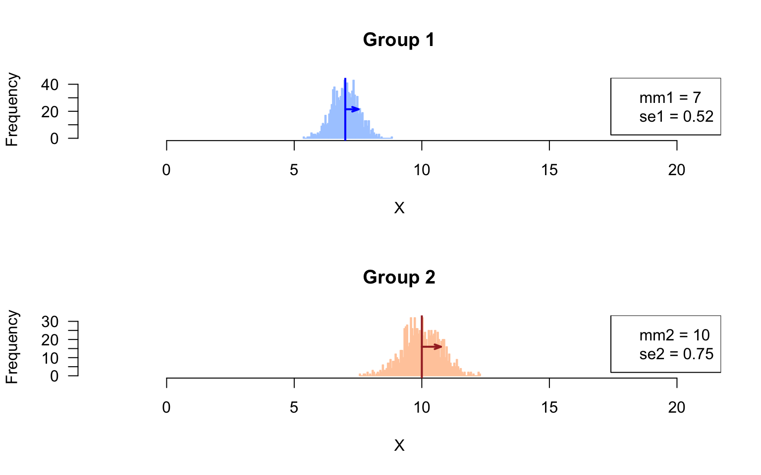
Sampling distribution of the mean
- Compare the standard deviations measures in the sampled values, and in the feature means. Do they differ ? Explain why.
Answer: the standard deviation of the sample means corresponds to the standard error.
Part 2: hypothesis testing
Run Student test on a given feature
Since we are interested by differences in either directions, we run a two-tailed test.
Hypotheses:
\[H_0: \mu_1 = \mu2\]
\[H_1: \mu_1 \ne \mu2\] Exercise: pick up a given feature (e.g. the \(267^{th}\)) and run a mean comparison test. Choose the parameters according to your experimental setting.
Tips:
t.test()- you need to choose the test depending on whether the two populations have equal variance (Student) or not (Welch). Since we defined different values for the populations standard deviations (\(\sigma_1\), \(\sigma_2\)), the choise is obvious.
i <- 267 ## Pick up a given feature, arbitrarily

## Select the values for this feature in the group 1 and group 2, resp.
## Tip: I use unlist() to convert a single-row data.frame into a vector
x1 <- unlist(group1[i, ])
x2 <- unlist(group2[i, ])

## Run Sudent t test on one pair of samples
t.result <- t.test(
  x = x1, y = x2,
  alternative = "two.sided", var.equal = FALSE)

## Print the result of the t test
print(t.result)
    Welch Two Sample t-test

data:  x1 and x2
t = -2.7572, df = 24.441, p-value = 0.01086
alternative hypothesis: true difference in means is not equal to 0
95 percent confidence interval:
 -3.8449347 -0.5546979
sample estimates:
mean of x mean of y
7.807264 10.007081 Interpret the result
The difference between sample means was \(d = 2.2\).
The \(t\) test computed the \(t\) statistics, which standardizes this observed distance between sample means relative to the estimated variance of the population, and to the sample sizes. With the random numbers generated above, the value is \(t_{obs} = -2.7572\).
The corresponding p-value is computed as the sum of the area of the left and right tails of the Student distribution, with \(\nu = n_1 + n_2 - 2 = 24.4411491\) degrees of freedom. It indicates the probability of obtaining by chance – under the null hypothesis – a result at least as extreme as the one we observed.
In our case, we obtain \(p = P(T > |t_{obs}| = P(T > 2.7572) = 0.0109\). This is higher than our threshold \(alpha = 0.05\). We thus accept the null hypothesis.
Replicating the test for each feature
In R, loops are quite inefficient, and it is generally recommended to directly run the computations on whole vectors (R has been designed to be efficient for this), or to use specific functions in order to apply a given function each row / column of a table, or to each element of a list.
For the sake of simplicity, we will first show how to implement a simple but inefficient code with a loop. In the advanced course (STATS2) will see how to optimize the speed with the apply() function.
## Define the statistics we want to collect
resultColumns <- c("i",       # iteration number
                    "m1",      # first sample mean
                    "m2",      # second sample mean
                    "s1",      # sd estimation for the first population
                    "s2",      # sd estimation for the second population
                    "d",       # difference between sample means
                    "t",       # test statistics
                    "df",      # degrees of freedom
                    "p.value"  # nominal p-value
                    )

## Instantiate a result table to store the results
resultTable <- data.frame(matrix(nrow = m, ncol = length(resultColumns)))
colnames(resultTable) <- resultColumns # set the column names
# View(resultTable) ## Check the table: it contians NA values

## Iterate random number sampling followed by t-tests
## Use the funciton system.time() to measure the elapsed time
## This function is particular: you can also use it with curly brackets in order to enclose a block of several lines
time.iteration <- system.time(
  for (i in 1:m) {
    ## Generate two vectors containing the values for sample 1 and sample 2, resp.
    x1 <- unlist(group1[i, ]) ## sample 1 values
    x2 <- unlist(group2[i, ]) ## sample 2 values

    ## Run the t test
    t.result <- t.test(
      x = x1, y = x2,
      alternative = "two.sided", var.equal = FALSE)
    # names(t.result)

    ## Collect the selected statistics in the result table
    resultTable[i, "i"] <- i
    resultTable[i, "t"] <- t.result$statistic
    resultTable[i, "df"] <- t.result$parameter
    resultTable[i, "p.value"] <- t.result$p.value

    ## Compute some additional statistics about the samples
    resultTable[i, "m1"] <- mean(x1) ## Mean of sample 1
    resultTable[i, "m2"] <- mean(x2) ## Mean of sample 2
    resultTable[i, "s1"] <- sd(x1) ## Standard dev estimation for population 1
    resultTable[i, "s2"] <- sd(x2) ## Standard dev estimation for population 1
    resultTable[i, "d"] <- resultTable[i, "m1"] - resultTable[i, "m2"]  ## Difference between sample means
  }
  #}
  ## View(resultTable)
)

print(time.iteration)
user system elapsed
0.846 0.292 1.107 Distribution of the observed differences for the \(1000\) iterations of the test
par(mfrow = c(2, 1))
#head(resultTable)

## Compute the maximal abslute value of difference to get a centered abcsissa.
## This enables to highlight whether the differences are positive or negative.
max.diff <- max(abs(resultTable$d))

## Draw an histogram of the observed differences
hist(resultTable$d,
     breaks = 100,
     col = "#DDFFEE",
     border = "#44DD88",
     las = 1,
     xlim = c(-max.diff, max.diff), ## Make sure that the graph is centered on 0
     main = "Differences between means",
     xlab = "Difference between means",
     ylab = "Number of tests")
abline(v = 0)

max.t <- max(abs(resultTable$t))
hist(resultTable$t,
     breaks = 100,
     col = "#DDFFEE",
     border = "#44DD88",
          las = 1,
     xlim = c(-max.t, max.t), ## Make sure that the graph is centered on 0
     main = "T statistics",
     xlab = "T-test statistic",
     ylab = "Number of tests")
abline(v = 0)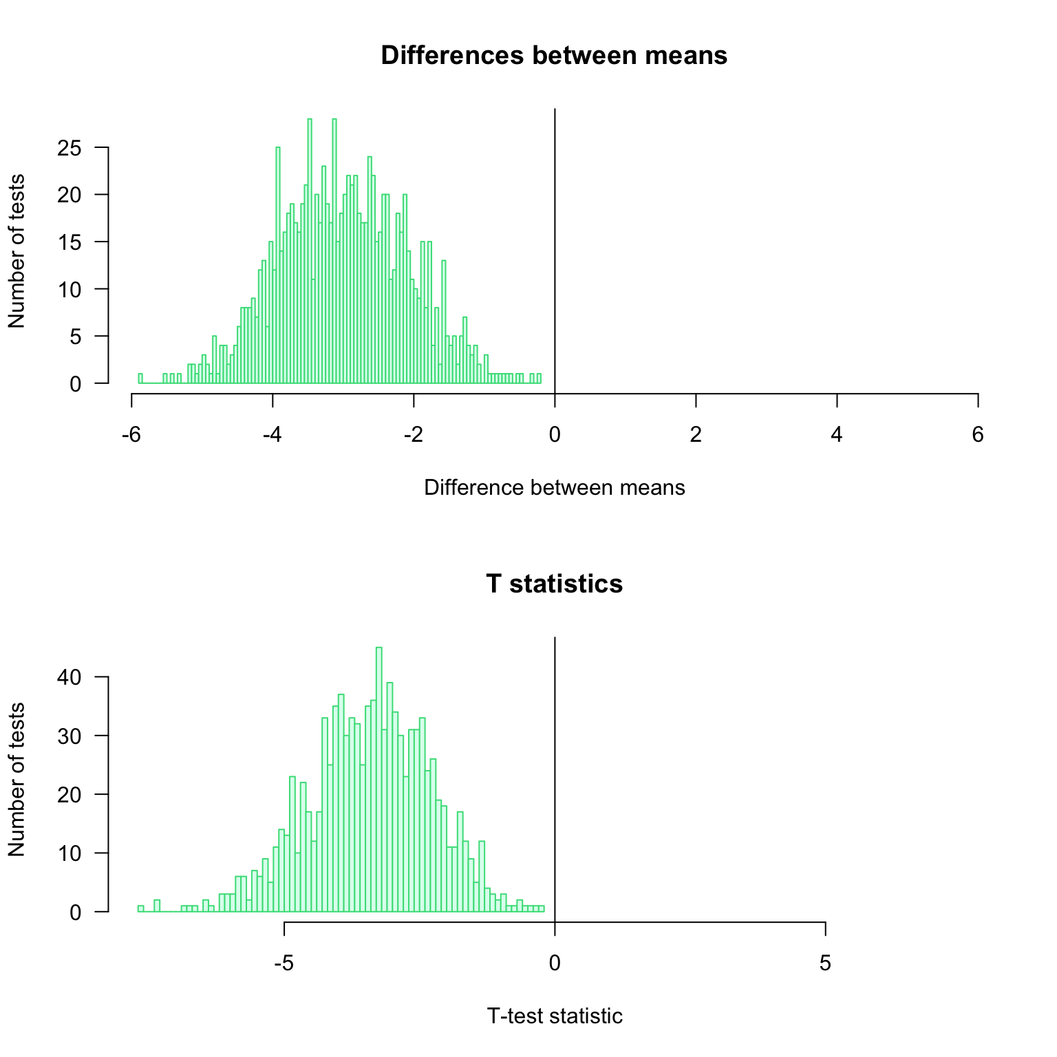
P-value histogram
## Choose a color depending on whether we are under H0 (grey) or H1 (pink)
if (mu1 == mu2) {
  histColor <- "#DDDDDD"
  histBorder <- "#888888"
} else {
  histColor <- "#FFCCCC"
  histBorder <- "#DD8888"
}

## Draw an histogram of p-values with 20 bins
hist(resultTable$p.value,
     breaks = 20,
     col = histColor,
     border = histBorder,
     las = 1,
     main = "P-value histogram",
     xlab = "T-test P-value",
     ylab = "Number of tests")

## Draw a horizontal line indicating the number of tests per bin that would be expected under null hypothesis
abline(h = m / 20, col = "darkgreen", lwd = 2)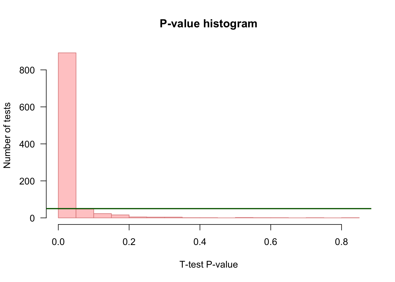
Creating a function to reuse the same code with different parameters
Depending on the selected task in the assignments above, we will run different tests with different parameters and compare the results. The most rudimentary way to do this is top copy-paste the chunk of code above for each test and set of parameters required for the assigned tasks.
However, having several copies of an almost identical block of code is a very bad pracrice in programming, for several reasons
- lack of readability: the code rapidly becomes very heavy;
- difficulty to maintain: any modification has to be done on each copy of the chunk of code;
- risk for consistency: this is a source of inconsistency, because at some moment we will modify one copy and forget another one.
A better practice is to define a function that encapsulates the code, and enables to modify the parameters by passing them as **arguments*. Hereafter we define a function that
takes the parameters of the analysis as arguments
- population means \(\mu_1\) and \(\mu_2\),
- population standard deviations \(\sigma_1\) and \(\sigma_2\),
- sample sizes \(n_1\) and \(n_2\),
- number of iterations \(r\).
- runs \(r\) iterations of the t-test with 2 random samples,
returns the results in a table with one row per iteration, and one column per resulting statistics (observed \(t\) score, p-value, difference between means, …);
#### Define a function that runs r iterations of the t-test ####

#' @title Repeat a T test with random numbers drawn from a normal distribution
#' @param mu1 mean of the first population
#' @param mu2 mean of the second population
#' @param sigma1 standard deviation of the first population
#' @param sigma2 standard deviation of the second population
#' @param n1 first sample size
#' @param n2 second sample size
#' @param m number of repetitions of the tests
#' @param ... additional parameters are passed to t.test(). This enables to set var.equal, alternative, ...
#' @return  a table with one row per repetition of the test, and one column per statistics
IterateTtest <- function(mu1,
                         mu2,
                         sigma1,
                         sigma2,
                         n1,
                         n2,
                         m,
                         ...) {


  ## Define the statistics we want to collect
  resultColumns <- c("i",       # iteration number
                      "m1",      # first sample mean
                      "m2",      # second sample mean
                      "s1",      # sd estimation for the first population
                      "s2",      # sd estimation for the second population
                      "d",       # difference between sample means
                      "t",       # test statistics
                      "df",      # degrees of freedom
                      "p.value"  # nominal p-value
  )

  ## Instantiate a result table to store the results
  resultTable <- data.frame(matrix(nrow = m, ncol = length(resultColumns)))
  colnames(resultTable) <- resultColumns # set the column names
  # View(resultTable) ## Check the table: it contians NA values

  ## Iterate random number sampling followed by t-tests
  for (i in 1:m) {
    ## Generate two vectors containing the values for sample 1 and sample 2, resp.
    x1 <- rnorm(n = n1, mean = mu1, sd = sigma1) ## sample 1 values
    x2 <- rnorm(n = n2, mean = mu2, sd = sigma2) ## sample 2 values

    ## Run the t test
    t.result <- t.test(
      x = x1, y = x2,
      alternative = "two.sided", var.equal = TRUE)
    # names(t.result)

    ## Collect the selected statistics in the result table
    resultTable[i, "i"] <- i
    resultTable[i, "t"] <- t.result$statistic
    resultTable[i, "df"] <- t.result$parameter
    resultTable[i, "p.value"] <- t.result$p.value

    ## Compute some additional statistics about the samples
    resultTable[i, "m1"] <- mean(x1) ## Mean of sample 1
    resultTable[i, "m2"] <- mean(x2) ## Mean of sample 2
    resultTable[i, "s1"] <- sd(x1) ## sd estimate for population 1
    resultTable[i, "s2"] <- sd(x2) ## sd estimate for population 2
    resultTable[i, "d"] <- resultTable[i, "m1"] - resultTable[i, "m2"] ## Difference between sample means
  }

  #### Compute multiple testing corrections ####

  ## E-value
  ## Expected number of FP
  resultTable$e.value <- resultTable$p.value * nrow(resultTable)

  ## Family-Wise Error Rate (FWER)
  ## Probability to have at least one FP given the p-value
  resultTable$FWER <- pbinom(q = 0,
                             size = nrow(resultTable),
                             prob = resultTable$p.value,
                             lower.tail = FALSE)


  ## Multiple testing corrections
  for (method in p.adjust.methods) {
    resultTable[, method] <- p.adjust(resultTable$p.value, method = method)
  }

  # ## Storey - Tibshirani q-value
  # qvalResult <- qvalue::qvalue(p = unlist(resultTable$p.value))
  # resultTable$q.value <-

  return(resultTable) ## This function returns the result table
}
We can now use this function to iterate the \(t\) test with the parameters we want. Let us measure the running time
## Some tests under H1
system.time(
  tTestTableH1 <- IterateTtest(mu1 = 7, mu2 = 10, sigma1 = 2, sigma2 = 3, n1 = 16, n2 = 16, m = 1000)
)
user system elapsed
0.598 0.247 0.817 ## Some tests under H0
system.time(
tTestTableH0 <- IterateTtest(mu1 = 10, mu2 = 10, sigma1 = 2, sigma2 = 3, n1 = 16, n2 = 16, m = 1000)
) user system elapsed
0.561 0.233 0.767 This function can then be used several times, with different values of the parameters.
## What happens when  the two means are equal (under the null hypothesis)
testH0 <- IterateTtest(mu1 = 10, mu2 = 10, sigma1 = sigma1, sigma2 = sigma2, n1 = n1, n2 = n2, m = m, var.equal = FALSE, alternative = "two.sided")


## Test increasing values of the difference between population means (delta)
delta0.1 <- IterateTtest(mu1 = mu1, mu2 = mu1 + 0.1, sigma1 = sigma1, sigma2 = sigma2, n1 = n1, n2 = n2, m = m, var.equal = FALSE, alternative = "two.sided")

delta0.5 <- IterateTtest(mu1 = mu1, mu2 = mu1 + 0.5, sigma1 = sigma1, sigma2 = sigma2, n1 = n1, n2 = n2, m = m, var.equal = FALSE, alternative = "two.sided")

delta1 <- IterateTtest(mu1 = mu1, mu2 = mu1 + 1, sigma1 = sigma1, sigma2 = sigma2, n1 = n1, n2 = n2, m = m, var.equal = FALSE, alternative = "two.sided")

delta2 <- IterateTtest(mu1 = mu1, mu2 = mu1 + 2, sigma1 = sigma1, sigma2 = sigma2, n1 = n1, n2 = n2, m = m, var.equal = FALSE, alternative = "two.sided")

delta3 <- IterateTtest(mu1 = mu1, mu2 = mu1 + 3, sigma1 = sigma1, sigma2 = sigma2, n1 = n1, n2 = n2, m = m, var.equal = FALSE, alternative = "two.sided")
P-value histograms
## Define a function that rdraws the p-value histogram
## based on the result table of t-test iterations
## as produced by the iterate.t.test() function.
pvalHistogram <- function(
  resultTable, ## required input (no default value): the result table from iterate.t.test()
  main = "P-value histogram",  ## main title (with default value)
  alpha = 0.05, ## Significance threshold
  ... ## Additional parameters, which will be passed to hist()
  ) {

  ## Plot the histogram
  hist(resultTable$p.value,
       breaks = seq(from = 0, to = 1, by = 0.05),
       las = 1,
       xlim = c(0,1),
       main = main,
       xlab = "T-test P-value",
       ylab = "Number of tests",
       ...)

  ## Draw a horizontal line indicating the number of tests per bin that would be expected under null hypothesis
  abline(h = m / 20, col = "darkgreen", lwd = 2)
  abline(v = alpha, col = "red", lwd = 2)

  ## Compute the percent of positive and negative results``
  nb.pos <- sum(resultTable$p.value < alpha)
  nb.neg <- m - nb.pos
  percent.pos <- 100 * nb.pos / m
  percent.neg <- 100 * nb.neg / m

  ## Add a legend indicating the percent of iterations declaed positive and negative, resp.
  legend("topright",
         bty = "o",
         bg = "white",
         cex = 0.7,
         legend = c(
           paste("m = ", nrow(resultTable)),
           paste("N(+) = ", nb.pos),
           paste("N(-) =", nb.neg),
           paste("pc(+) = ", round(digits = 2, percent.pos)),
           paste("pc(-) =", round(digits = 2, percent.neg))
         ))
}par(mfrow = c(3, 2)) ## Prepare 2 x 2 panels figure
pvalHistogram(testH0, main = "under H0 (mu1 = mu2)", col = "#DDDDDD", border = "#DDDDDD")
pvalHistogram(delta0.1, main = "mu1 - mu2 = 0.1", col = "#FFDDBB")
pvalHistogram(delta0.5, main = "mu1 - mu2 = 0.5", col = "#FFDDBB")
pvalHistogram(delta1, main = "mu1 - mu2 = 1", col = "#FFDDBB")
pvalHistogram(delta2, main = "mu1 - mu2 = 2", col = "#FFDDBB")
pvalHistogram(delta3, main = "mu1 - mu2 = 3", col = "#FFDDBB")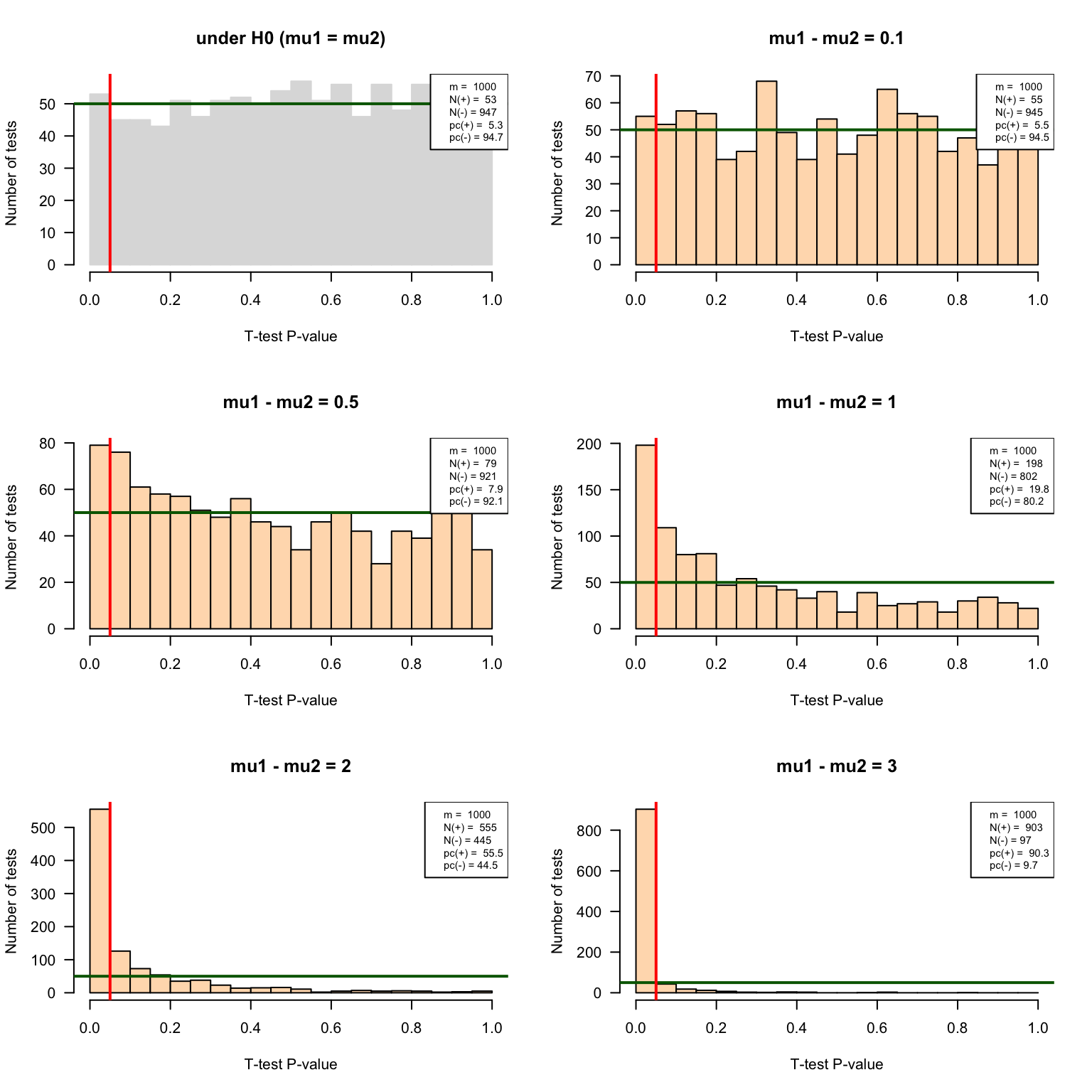
P-value historams of the multiple test results with increasing effect sizes.
Volcano plots
#### Define VolcanoPlot() function ####
VolcanoPlot <- function(resultTable,
                        alpha = 0.05,
                        ...) {


  ## Collect effect size values for the X axis
  effectSize <- resultTable$d
  maxXabs <- max(abs(effectSize))
  xmax <- signif(digits = 1, maxXabs)

  ## Collect p-values for the Y axis
  log10Pval <- -log10(resultTable$p.value)

  plot(effectSize,
       log10Pval,
       xlim = c(-xmax, xmax),
       lax = 1,
       xlab = "Effect size",
       ylab = "-log10(Pval)",
       ...
       )
  abline(v = 0)
  abline(h = 0)
  abline(h = -log10(alpha), col = "red")

  ## Compute the percent of positive and negative results``
  nb.pos <- sum(resultTable$p.value < alpha)
  nb.neg <- m - nb.pos
  percent.pos <- 100 * nb.pos / m
  percent.neg <- 100 * nb.neg / m


  ## Add a legend indicating the percent of iterations declaed positive and negative, resp.
  legend("topright",
         bty = "o",
         bg = "white",
         cex = 0.7,
         legend = c(
           paste("m = ", nrow(resultTable)),
           paste("N(+) = ", nb.pos),
           paste("N(-) =", nb.neg),
           paste("pc(+) = ", round(digits = 2, percent.pos)),
           paste("pc(-) =", round(digits = 2, percent.neg))
         ))

}par(mfrow = c(3,2))
VolcanoPlot(testH0, main = "under H0 (mu1 = mu2)", col = "#DDDDDD")
VolcanoPlot(delta0.1, main = "mu1 - mu2 = 0.1", col = "#FFDDBB")
VolcanoPlot(delta0.5, main = "mu1 - mu2 = 0.5", col = "#FFDDBB")
VolcanoPlot(delta1, main = "mu1 - mu2 = 1", col = "#FFDDBB")
VolcanoPlot(delta2, main = "mu1 - mu2 = 2", col = "#FFDDBB")
VolcanoPlot(delta3, main = "mu1 - mu2 = 3", col = "#FFDDBB")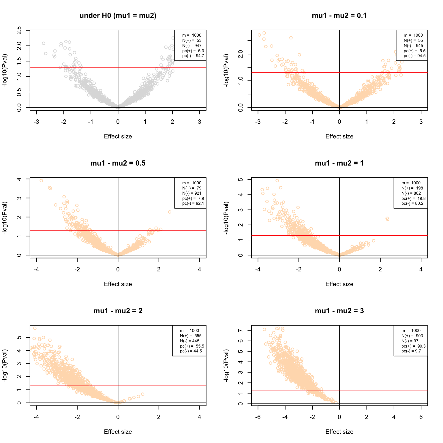
Volcano plots of the multiple test results with increasing effect sizes.
Multiple testing corrections
par(mfrow = c(3,2))

MultiCorrectionsPlot <- function(resultTable,
                                 main = "Multiple testing corrections") {
  #### Compare p-value corrections under H0 ####
  plot(resultTable$p.value,
       resultTable$p.value,
       main = main,
       col = "grey",
       log = "xy",
       xlab = "Nominal P-value",
       ylab = "Corrected P-value",
       panel.first = grid())
  abline(v = c(0,1))
  abline(h = c(0,1))
  abline(h  = alpha, col = "red")
  abline(v  = alpha, col = "red")

  ## FWER
  points(resultTable$p.value,
         resultTable$FWER, col = "blue")

  ## Bonferroni correction
  points(resultTable$p.value,
         resultTable$bonferroni, col = "orange")

  ## Benjamini-Hochberg
  points(resultTable$p.value,
         resultTable$BH, col = "darkgreen")
}


MultiCorrectionsPlot(testH0, main = "under H0 (mu1 = mu2)")
MultiCorrectionsPlot(delta0.1, main = "mu1 - mu2 = 0.1")
MultiCorrectionsPlot(delta0.5, main = "mu1 - mu2 = 0.5")
MultiCorrectionsPlot(delta1, main = "mu1 - mu2 = 1")
MultiCorrectionsPlot(delta2, main = "mu1 - mu2 = 2")
MultiCorrectionsPlot(delta3, main = "mu1 - mu2 = 3")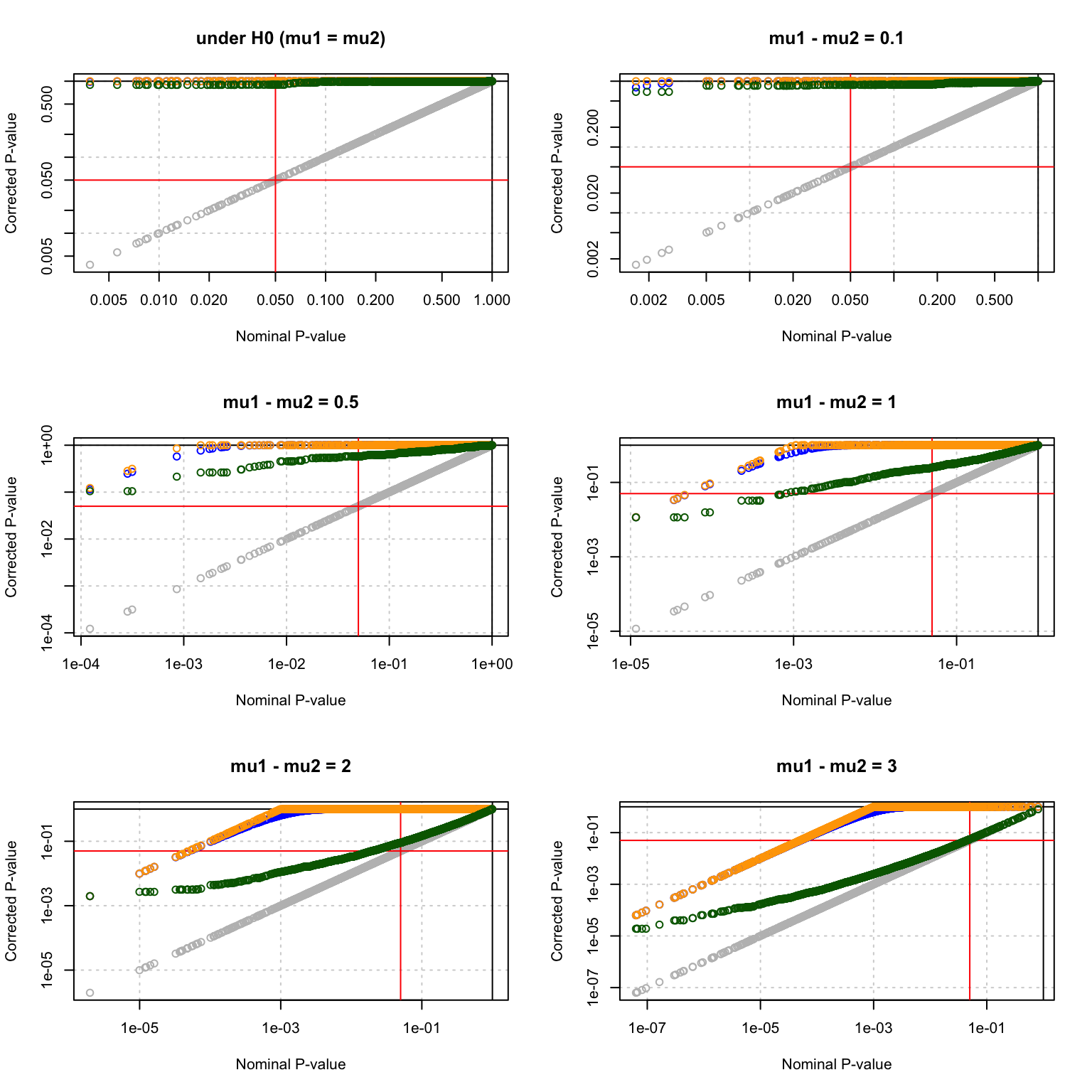
Multiple testing corrections.
```
Interpretation of the results
We should now write a report of interpretation, which will address the following questions.
Based on the experiments under \(H_0\), compute the number of false positives and estimate the false positive rate (FPR). Compare these values with the E-value (expected number of false positives) for the 1000 tests, and with your \(alpha\) trheshold.
Based on the experiments under \(H_1\), estimate the sensitivity (Sn) of the test for the different mean differences tested here.
Interpret the histograms of P-values obtained with the different parameters ?
Draw a power curve (i.e. the sensitivity as a function of the actual difference between population means)
Discuss about the adequation between the test and the conditions of our simulations.
Do these observations correspond to what would be expected from the theory?