Principal Component Analysis of multi-omics data (Pavkovic 2019)
Jacques van Helden
2020-06-04 09:05:22
Introduction
La valeur de 2 + 2 est 4.
On peut aussi insérer du bash:
#### Example of bash code running in an R notebook ####

echo Hello World

## Run the Linux command whoami
whoami

## Run echo with an embedded result of the whoami command
echo "I am `whoami`"
Hello World
jvanhelden
I am jvanheldenMaterial and methods
#### Example of R chunk ####

## The variable defined in the previous chunk s still in the environment for the next chunks
print(a)
Data
##### Load the data ####

## Note: this path is only valid if you are working on the IFB core cluster.
## If not, it should point to the folder where you downloaded the memory image from the github repository
#load('/shared/projects/dubii2020/data/module3/seance5/pavkovic2019_proteome_uuo_memimage.Rdata')
#load('/shared/projects/dubii2020/data/module3/seance5/pavkovic2019_transcriptome_fa_memimage.Rdata')
load('/shared/projects/dubii2020/data/module3/seance5/pavkovic2019_proteome_fa_memimage.Rdata')

kable(t(as.data.frame(parameters)),
      col.names = "Parameter",
caption = "Parameters used for this analysis")| Parameter | |
|---|---|
| datatype | proteome |
| dataset | fa |
| epsilon | 0.1 |
| forceDownload | FALSE |
| undetectedLimit | 100 |
| filePrefix | pavkovic2019_proteome_fa_ |
#### Choose the non-normalised filtered log2 data to play with ####
# x <- log2MedianCentered
x <- log2Standardized
dim(x) # Check the dimensions
[1] 8044 10 [1] "normal_1" "normal_2" "day1_1" "day1_2" "day2_1" "day2_2" "day7_1" "day7_2" "day14_1" "day14_2" ## Print the first rows of the data matrix to check the content
kable(head(x), caption = "First rows of the data matrix")| normal_1 | normal_2 | day1_1 | day1_2 | day2_1 | day2_2 | day7_1 | day7_2 | day14_1 | day14_2 | |
|---|---|---|---|---|---|---|---|---|---|---|
| ENSMUSG00000037686 | 9.074107 | 9.004221 | 8.396524 | 8.460642 | 7.543358 | 7.898095 | 7.408463 | 7.611362 | 7.594110 | 7.924550 |
| ENSMUSG00000027831 | 7.867928 | 7.784098 | 7.459918 | 7.428059 | 7.799405 | 7.640674 | 7.697335 | 7.819737 | 7.833291 | 7.280241 |
| ENSMUSG00000039201 | 4.919638 | 4.769868 | 5.856594 | 5.695505 | 6.250616 | 6.111805 | 5.325407 | 5.004578 | 4.812991 | 5.057171 |
| ENSMUSG00000031095 | 11.979430 | 11.722994 | 11.998335 | 11.883829 | 12.161338 | 12.170381 | 12.009147 | 12.243316 | 12.037636 | 12.029025 |
| ENSMUSG00000034931 | 9.769235 | 9.674498 | 9.843766 | 9.879726 | 9.923981 | 9.936608 | 10.043512 | 9.928562 | 9.915093 | 9.819190 |
| ENSMUSG00000038208 | 6.243681 | 6.303451 | 5.860863 | 6.404236 | 6.307760 | 6.355272 | 6.636115 | 6.641220 | 6.392972 | 6.170323 |
Results
PCA
#### Compute the components ####
## Beware: the individuals should come as row --> we have to transpose the expression matrix
res.pca <- PCA(t(x), scale.unit = FALSE, ncp = ncol(x), graph = FALSE)

## Check the content of the resulting object
# names(res.pca)

## Eigen values
kable(res.pca$eig, caption = "Eigen values of the PCs")| eigenvalue | percentage of variance | cumulative percentage of variance | |
|---|---|---|---|
| comp 1 | 606.51636 | 56.306102 | 56.30610 |
| comp 2 | 251.71246 | 23.367791 | 79.67389 |
| comp 3 | 67.43145 | 6.260016 | 85.93391 |
| comp 4 | 44.90736 | 4.168986 | 90.10290 |
| comp 5 | 26.20929 | 2.433146 | 92.53604 |
| comp 6 | 24.37324 | 2.262696 | 94.79874 |
| comp 7 | 22.35638 | 2.075460 | 96.87420 |
| comp 8 | 18.43731 | 1.711632 | 98.58583 |
| comp 9 | 15.23312 | 1.414170 | 100.00000 |
## Variables versus components
kable(head(res.pca$var$coord), caption = "Coordonates of the features in the PC space") | Dim.1 | Dim.2 | Dim.3 | Dim.4 | Dim.5 | Dim.6 | Dim.7 | Dim.8 | Dim.9 | |
|---|---|---|---|---|---|---|---|---|---|
| ENSMUSG00000037686 | 0.5602567 | -0.0695260 | 0.0829844 | 0.0230604 | -0.0244854 | -0.0529326 | 0.0175894 | -0.0545825 | 0.0312909 |
| ENSMUSG00000027831 | -0.0268473 | -0.0428831 | 0.1005814 | 0.1174449 | -0.0299994 | -0.0266777 | 0.0007058 | 0.0157059 | -0.0949374 |
| ENSMUSG00000039201 | -0.0638299 | 0.5087985 | -0.0664831 | 0.0348704 | 0.0387480 | 0.0533996 | -0.0583329 | 0.0239771 | 0.0220538 |
| ENSMUSG00000031095 | -0.1030284 | 0.0446238 | -0.0159905 | 0.0159499 | 0.0210804 | -0.0439426 | -0.0188236 | -0.0548504 | -0.0362927 |
| ENSMUSG00000034931 | -0.0852404 | 0.0316188 | 0.0253286 | -0.0069091 | 0.0108797 | 0.0140832 | -0.0025666 | -0.0032059 | 0.0128727 |
| ENSMUSG00000038208 | -0.1338140 | -0.0516643 | 0.0725614 | 0.0786191 | -0.0445291 | -0.0110313 | 0.0894065 | -0.0079813 | 0.0574955 |
# head(res.pca$var$cor) ## Correlation
# head(res.pca$var$cos2) ## Cos2 (squared correlation)
# head(res.pca$var$contrib) ## Contribution of each variable to each component (loading ?)

## Check that Cos2 is just the square of the correlation
# head(res.pca$var$cos2) - head(res.pca$var$cor)^2

## The sum of squared correlations per variable must be 1
# head(apply(res.pca$var$cos2, 1, sum))


## Individuals versus components
kable(res.pca$ind$coord, caption = "Coordinates of the individuals in the variable space") ## Coordinates| Dim.1 | Dim.2 | Dim.3 | Dim.4 | Dim.5 | Dim.6 | Dim.7 | Dim.8 | Dim.9 | |
|---|---|---|---|---|---|---|---|---|---|
| normal_1 | 34.420376 | -10.595090 | 9.6091387 | 6.2102260 | 5.6634490 | 0.6509477 | -1.2740605 | -7.1291849 | -2.145107 |
| normal_2 | 37.996171 | -16.459654 | -2.4550846 | 5.6725013 | -8.4996304 | -0.7169252 | 0.0193776 | 5.9068331 | 1.014266 |
| day1_1 | 20.160709 | 17.358313 | 1.0450993 | -13.4644331 | -2.6142332 | 0.2919571 | -6.9089453 | -0.0249585 | -3.218958 |
| day1_2 | 16.470097 | 15.509316 | 3.6790390 | -5.7959211 | 1.7879874 | 1.2732947 | 10.8538757 | 0.5453522 | 4.229374 |
| day2_1 | -12.892119 | 22.418951 | -7.7540613 | 9.2511401 | -0.5073773 | 5.9126144 | 1.9212908 | 0.6999172 | -5.913915 |
| day2_2 | -8.627622 | 19.783561 | -0.2922252 | 6.7979005 | 3.7748811 | -8.3590432 | -4.8463322 | 1.9211309 | 4.984201 |
| day7_1 | -33.508194 | -6.391523 | 10.0724149 | 0.3733335 | -2.9401694 | 8.5632004 | -3.6773246 | -0.0612934 | 4.836156 |
| day7_2 | -30.738656 | -6.669942 | 0.9637777 | -1.3423506 | -7.6873175 | -7.3442106 | 3.5574998 | -5.8294952 | -2.257436 |
| day14_1 | -21.118523 | -18.444311 | 4.5701275 | -3.6995666 | 7.0523093 | -2.2516599 | 1.3980362 | 7.0997749 | -4.571015 |
| day14_2 | -2.162239 | -16.509621 | -19.4382259 | -4.0028299 | 3.9701011 | 1.9798247 | -1.0434173 | -3.1280762 | 3.042433 |
Eigen values plot
#### Plot eigen values ####
fviz_eig(res.pca, addlabels = TRUE, ylim = c(0, 50), main = paste(parameters$datatype, parameters$dataset))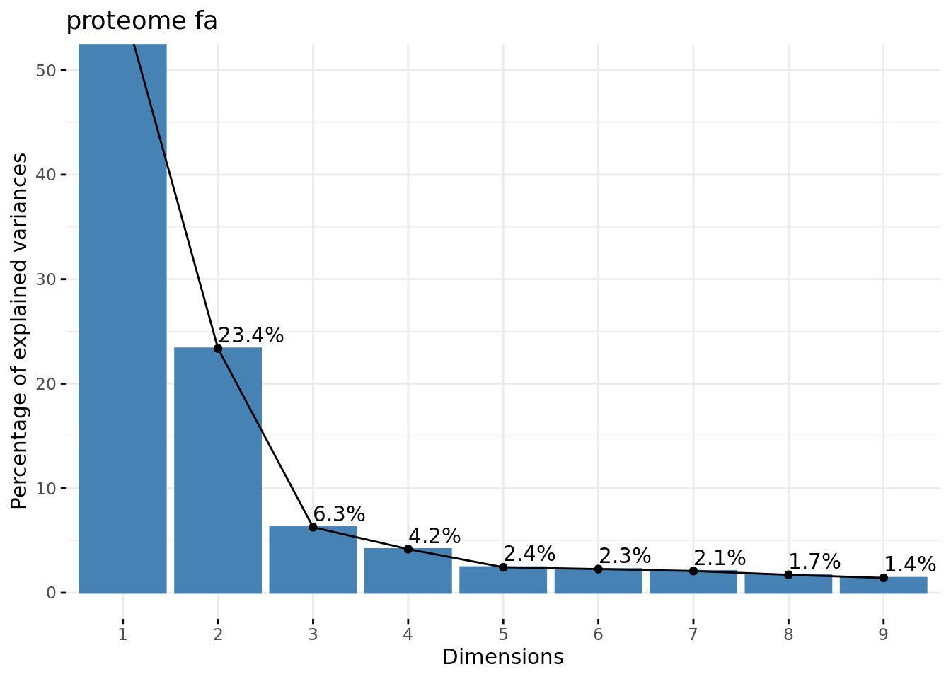
Eigenvalues plot.
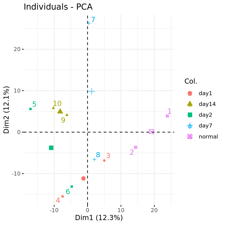
#### Plot PC1 vs PC2 with condition-specific colors ####
fviz_pca_ind(res.pca, axes = c(1,2),
             col.ind = metadata$condition,
             repel = TRUE # Avoid overlap between labels
)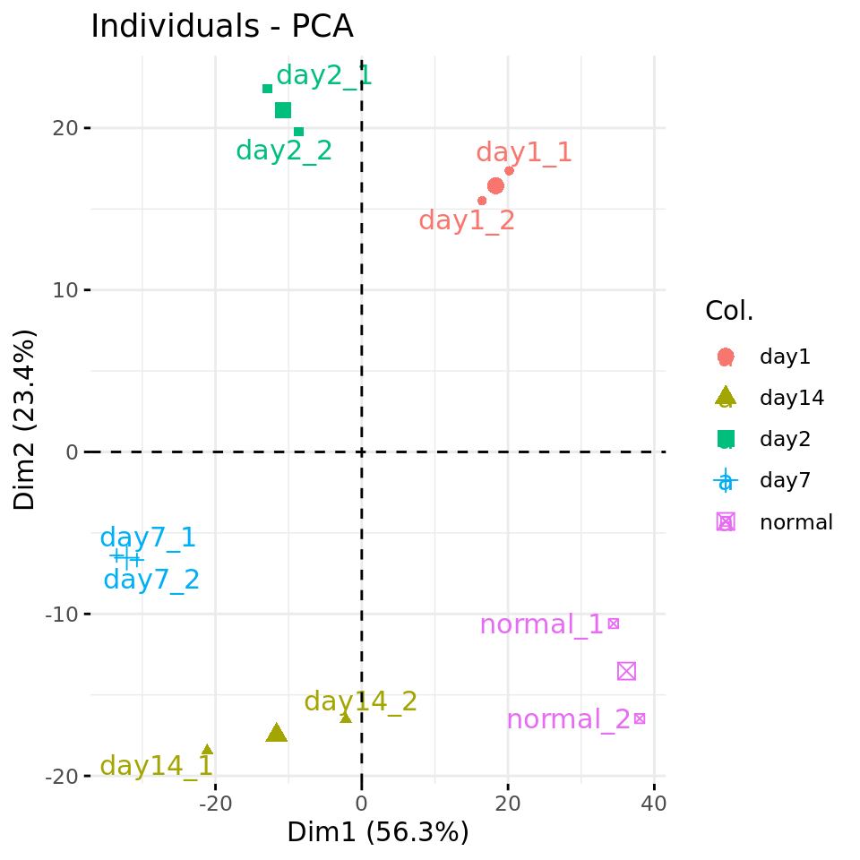
PC plots of the dataset proteome fa
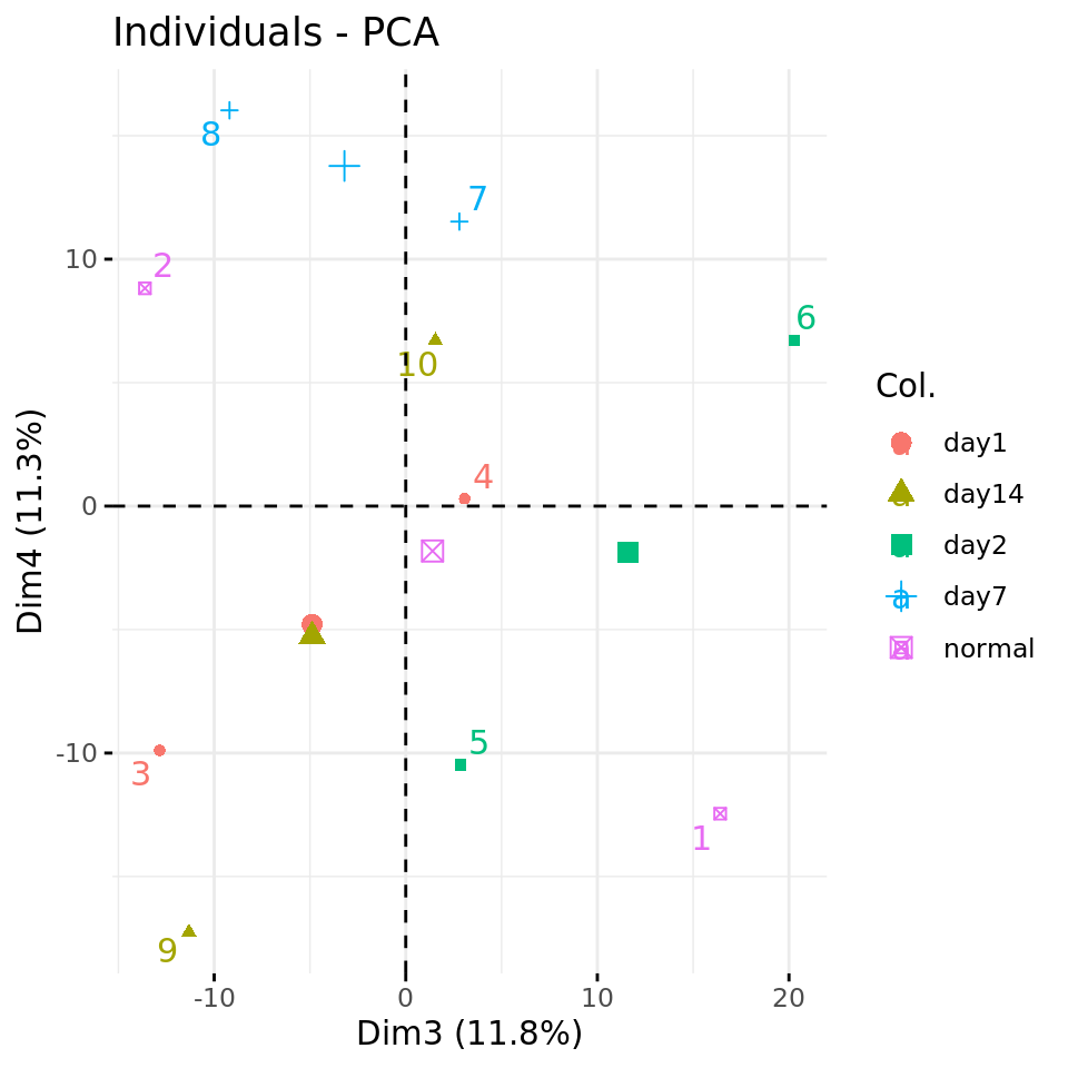
#### Plot PC4 vs PC3 with condition-specific colors ####
fviz_pca_ind(res.pca, axes = c(3,4),
             col.ind = metadata$condition,
             repel = TRUE # Avoid overlap between labels
)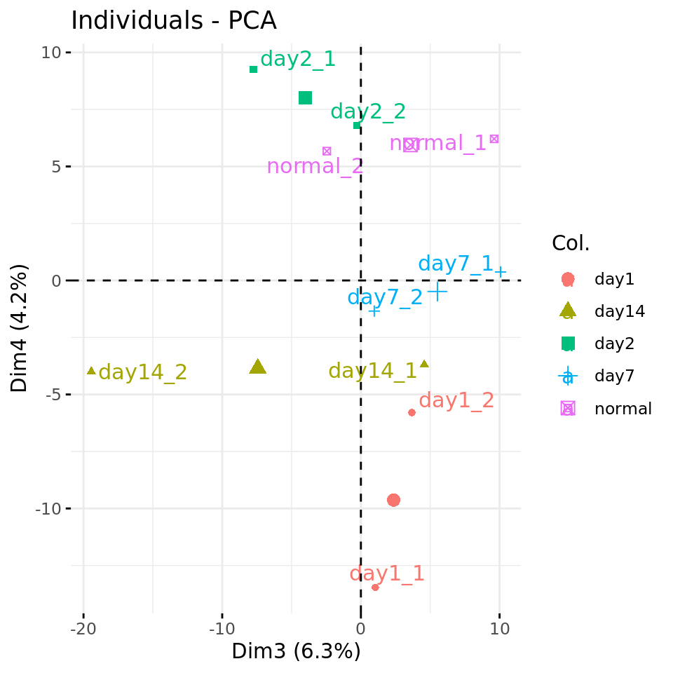
PC plots of the dataset proteome fa
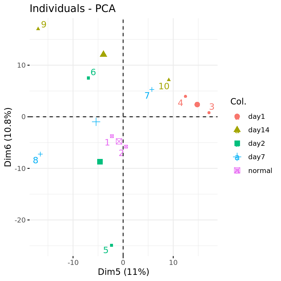
#### Plot PC5 vs PC6 with condition-specific colors ####
fviz_pca_ind(res.pca, axes = c(5, 6),
             col.ind = metadata$condition,
             repel = TRUE # Avoid overlap between labels
)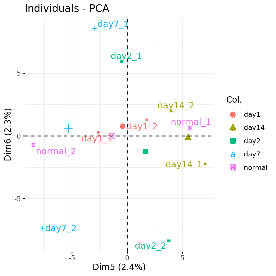
PC plots of the dataset proteome fa
Nous observons une excellente cohérence entre répliques.
Les 2 premières composantes capturent visiblement une progression temporelle, qui se manifeste par une répartition cyclique.
Negative control
We would like to check that the structuration of differs from what would be expected by chance. For this, we can use an empirical approach: randomise the dataset by shuffling its values, and run the PCA again.
Shuffled matrix
The simplest wway to do this is to shufle all the values of the table, by applying the command sample() on the data frame x.
#### Negatve control: permute all the values of the data matrix ####

## Shuffle all the values of the data matrix
shuffledValues <- sample(unlist(x) , size = prod(dim(x)), replace = FALSE) # This gives a vector

## Place the shuffled values in a matrix of the same dimensions as the oroginal data matrix
xShuffled <- matrix(
  data = shuffledValues,
  nrow = nrow(x), ncol = ncol(x))
table(xShuffled == x) ## the values match on average one time per permutation
FALSE  TRUE
80437     3
## Check that the original expressio matrix has high correlation values betwen individuals
xCor <- cor(x)
rownames(xCor) <- colnames(x)
colnames(xCor) <- colnames(x)
kable(cor(x),
caption = "Correlation between columns (samples) of the original expression matrix. ",
row.names = TRUE)| normal_1 | normal_2 | day1_1 | day1_2 | day2_1 | day2_2 | day7_1 | day7_2 | day14_1 | day14_2 | |
|---|---|---|---|---|---|---|---|---|---|---|
| normal_1 | 1.0000000 | 0.9919038 | 0.9779548 | 0.9796817 | 0.9471940 | 0.9564886 | 0.9328708 | 0.9347125 | 0.9513990 | 0.9668757 |
| normal_2 | 0.9919038 | 1.0000000 | 0.9726016 | 0.9728881 | 0.9395325 | 0.9471756 | 0.9234387 | 0.9284722 | 0.9453908 | 0.9685007 |
| day1_1 | 0.9779548 | 0.9726016 | 1.0000000 | 0.9935187 | 0.9747140 | 0.9801014 | 0.9474768 | 0.9507433 | 0.9542045 | 0.9682995 |
| day1_2 | 0.9796817 | 0.9728881 | 0.9935187 | 1.0000000 | 0.9793634 | 0.9835448 | 0.9541723 | 0.9570625 | 0.9605813 | 0.9708474 |
| day2_1 | 0.9471940 | 0.9395325 | 0.9747140 | 0.9793634 | 1.0000000 | 0.9933910 | 0.9753701 | 0.9772008 | 0.9691986 | 0.9710011 |
| day2_2 | 0.9564886 | 0.9471756 | 0.9801014 | 0.9835448 | 0.9933910 | 1.0000000 | 0.9756376 | 0.9779807 | 0.9727696 | 0.9720635 |
| day7_1 | 0.9328708 | 0.9234387 | 0.9474768 | 0.9541723 | 0.9753701 | 0.9756376 | 1.0000000 | 0.9932936 | 0.9901542 | 0.9715261 |
| day7_2 | 0.9347125 | 0.9284722 | 0.9507433 | 0.9570625 | 0.9772008 | 0.9779807 | 0.9932936 | 1.0000000 | 0.9906668 | 0.9772792 |
| day14_1 | 0.9513990 | 0.9453908 | 0.9542045 | 0.9605813 | 0.9691986 | 0.9727696 | 0.9901542 | 0.9906668 | 1.0000000 | 0.9841713 |
| day14_2 | 0.9668757 | 0.9685007 | 0.9682995 | 0.9708474 | 0.9710011 | 0.9720635 | 0.9715261 | 0.9772792 | 0.9841713 | 1.0000000 |
## Check that the permuted matrix is not correlated anymore
## Inter-sample correlations should be around 0 except in the diagonal
xShuffledCor <- cor(xShuffled)
rownames(xShuffledCor) <- paste0("shufMat", 1:ncol(xShuffledCor))
colnames(xShuffledCor) <- paste0("shufMat", 1:ncol(xShuffledCor))
kable(xShuffledCor,
      caption = "Correlation between columns of the shuffled expression matrix",
row.names = TRUE)| shufMat1 | shufMat2 | shufMat3 | shufMat4 | shufMat5 | shufMat6 | shufMat7 | shufMat8 | shufMat9 | shufMat10 | |
|---|---|---|---|---|---|---|---|---|---|---|
| shufMat1 | 1.0000000 | -0.0248187 | -0.0005062 | 0.0167536 | 0.0078892 | -0.0068962 | -0.0176948 | 0.0167558 | -0.0043146 | 0.0017627 |
| shufMat2 | -0.0248187 | 1.0000000 | -0.0129004 | 0.0022150 | 0.0020933 | -0.0065190 | 0.0013577 | -0.0039026 | -0.0062836 | 0.0056548 |
| shufMat3 | -0.0005062 | -0.0129004 | 1.0000000 | -0.0075904 | -0.0167126 | 0.0047331 | -0.0194989 | -0.0009989 | -0.0058640 | -0.0128864 |
| shufMat4 | 0.0167536 | 0.0022150 | -0.0075904 | 1.0000000 | -0.0105706 | -0.0264597 | -0.0013484 | 0.0015994 | 0.0034866 | -0.0036453 |
| shufMat5 | 0.0078892 | 0.0020933 | -0.0167126 | -0.0105706 | 1.0000000 | -0.0090114 | 0.0188795 | 0.0128834 | 0.0116799 | -0.0077141 |
| shufMat6 | -0.0068962 | -0.0065190 | 0.0047331 | -0.0264597 | -0.0090114 | 1.0000000 | 0.0008281 | 0.0068692 | -0.0122195 | -0.0039007 |
| shufMat7 | -0.0176948 | 0.0013577 | -0.0194989 | -0.0013484 | 0.0188795 | 0.0008281 | 1.0000000 | 0.0136776 | 0.0038547 | 0.0169533 |
| shufMat8 | 0.0167558 | -0.0039026 | -0.0009989 | 0.0015994 | 0.0128834 | 0.0068692 | 0.0136776 | 1.0000000 | 0.0045827 | -0.0113638 |
| shufMat9 | -0.0043146 | -0.0062836 | -0.0058640 | 0.0034866 | 0.0116799 | -0.0122195 | 0.0038547 | 0.0045827 | 1.0000000 | -0.0031171 |
| shufMat10 | 0.0017627 | 0.0056548 | -0.0128864 | -0.0036453 | -0.0077141 | -0.0039007 | 0.0169533 | -0.0113638 | -0.0031171 | 1.0000000 |
## Compute the Principal Components on the shuffled
xShuffledPCA <- PCA(t(xShuffled), scale.unit = FALSE, ncp = ncol(x), graph = FALSE)
#### Eigen values ####
fviz_eig(xShuffledPCA, addlabels = TRUE, ylim = c(0, 50),
main = paste("Shuffled matrix from", parameters$datatype, parameters$dataset))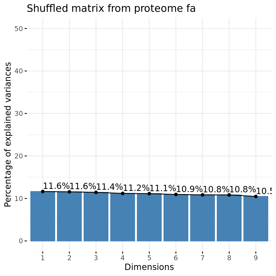
Negative control 1: eigen values of PCs from a data matrix with shuffled values.
#### Plot PC1 vs PC2 with condition-specific colors ####
fviz_pca_ind(xShuffledPCA, axes = c(1,2),
             col.ind = metadata$condition,
             repel = TRUE # Avoid overlap between labels
)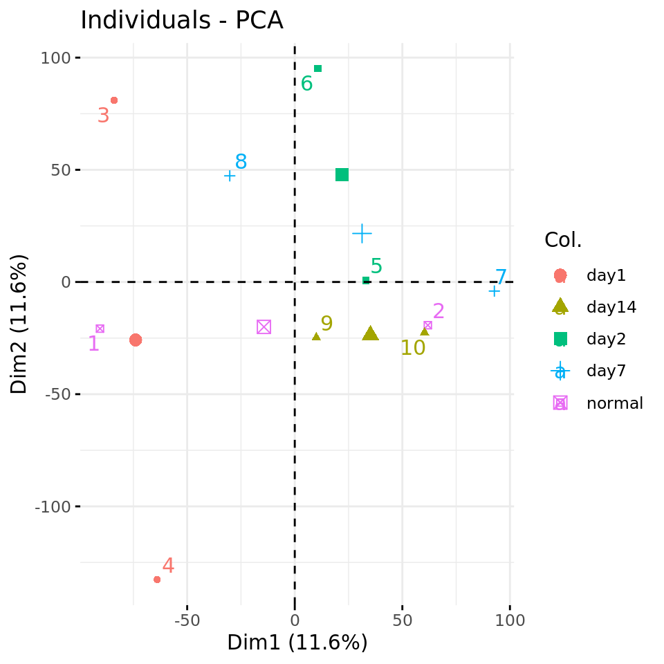
Negative control 1: PC plots from a data matrix with shuffled values.
#### Plot PC4 vs PC3 with condition-specific colors ####
fviz_pca_ind(xShuffledPCA, axes = c(3,4),
             col.ind = metadata$condition,
             repel = TRUE # Avoid overlap between labels
)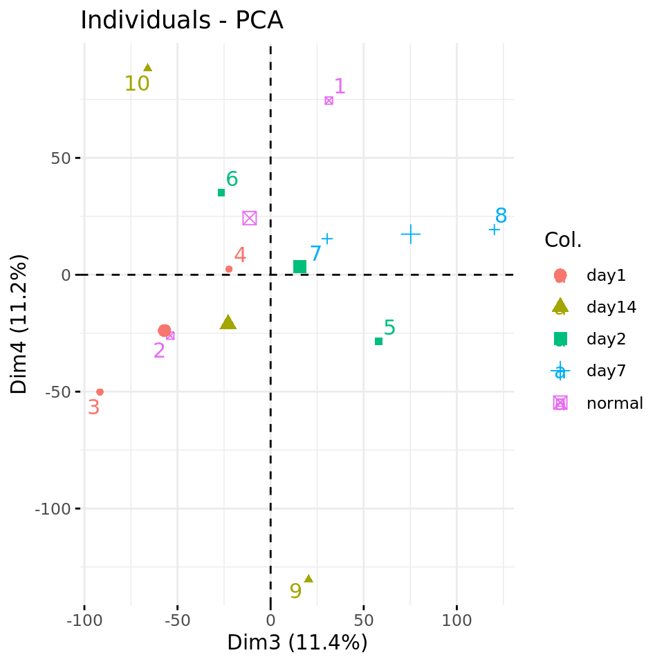
Negative control 1: PC plots from a data matrix with shuffled values.
#### Plot PC5 vs PC6 with condition-specific colors ####
fviz_pca_ind(xShuffledPCA, axes = c(5, 6),
             col.ind = metadata$condition,
             repel = TRUE # Avoid overlap between labels
)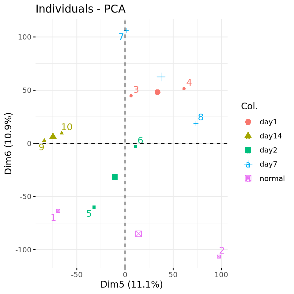
Negative control 1: PC plots from a data matrix with shuffled values.
Row-wise shuffled matrix
A more refined appoach is to shuffle the values inside each row of the x data frame, by cmbining apply() and sample().
Note that this approach will preserve a quite high correlation between the columns of the matrix, which will reflect the gene-specific level of expressions (some genes have very high levels across all conditons, and some others very low levels across all conditions). However the values will now be sampled independently of the studied factor (the impact of the time point). Consequently, the row-wise shuffled matrix will have data distributions that better reflects those of biological data, so that this control can be considered as a more suitable than the whole matrix shuffling.
#### Negative control : row-wise permutations of the values ####

## Permute values inside each row of the matrix
xShuffledRows <- t(apply(x, 1, sample))
dim(xShuffledRows)
[1] 8044 10
FALSE  TRUE
72317  8123
## Check that therow-wise means are the same between
xRowMeans <- apply(x, 1, mean)
shuffledRowMeans <- apply(xShuffledRows, 1, mean)
plot(xRowMeans, shuffledRowMeans)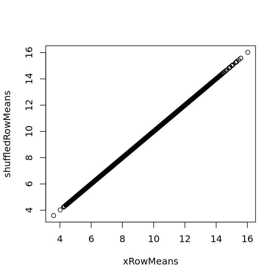
Row-wise shuffling of the values removes the sample-specific information whilst preserving the mean of each feature.
TRUE
8044
## Check the correlation nbetween columns of the row-wise permuted matrix.
## Note: values canbe high if the rows have very different ranges (which is the case here)
xShuffledRowsCor <- cor(xShuffledRows)
rownames(xShuffledRowsCor) <- paste("shufRow", 1:ncol(xShuffledRowsCor))
colnames(xShuffledRowsCor) <- paste("shufRow", 1:ncol(xShuffledRowsCor))
kable(xShuffledRowsCor,
caption = "Correlation between columns of the row-wise shuffled expression matrix",
row.names = TRUE) ## Inter-sample correlations should be around 0 except in the diagonal| shufRow 1 | shufRow 2 | shufRow 3 | shufRow 4 | shufRow 5 | shufRow 6 | shufRow 7 | shufRow 8 | shufRow 9 | shufRow 10 | |
|---|---|---|---|---|---|---|---|---|---|---|
| shufRow 1 | 1.0000000 | 0.9662502 | 0.9662541 | 0.9655092 | 0.9646211 | 0.9658989 | 0.9657678 | 0.9653788 | 0.9651178 | 0.9656101 |
| shufRow 2 | 0.9662502 | 1.0000000 | 0.9680615 | 0.9668726 | 0.9653749 | 0.9658288 | 0.9662572 | 0.9678591 | 0.9663942 | 0.9668575 |
| shufRow 3 | 0.9662541 | 0.9680615 | 1.0000000 | 0.9684497 | 0.9665600 | 0.9659214 | 0.9660011 | 0.9671768 | 0.9673919 | 0.9676081 |
| shufRow 4 | 0.9655092 | 0.9668726 | 0.9684497 | 1.0000000 | 0.9672470 | 0.9683681 | 0.9652249 | 0.9674407 | 0.9667318 | 0.9689265 |
| shufRow 5 | 0.9646211 | 0.9653749 | 0.9665600 | 0.9672470 | 1.0000000 | 0.9664240 | 0.9664619 | 0.9662762 | 0.9670899 | 0.9680278 |
| shufRow 6 | 0.9658989 | 0.9658288 | 0.9659214 | 0.9683681 | 0.9664240 | 1.0000000 | 0.9653366 | 0.9667213 | 0.9658113 | 0.9673918 |
| shufRow 7 | 0.9657678 | 0.9662572 | 0.9660011 | 0.9652249 | 0.9664619 | 0.9653366 | 1.0000000 | 0.9660601 | 0.9661718 | 0.9685299 |
| shufRow 8 | 0.9653788 | 0.9678591 | 0.9671768 | 0.9674407 | 0.9662762 | 0.9667213 | 0.9660601 | 1.0000000 | 0.9667838 | 0.9676198 |
| shufRow 9 | 0.9651178 | 0.9663942 | 0.9673919 | 0.9667318 | 0.9670899 | 0.9658113 | 0.9661718 | 0.9667838 | 1.0000000 | 0.9676061 |
| shufRow 10 | 0.9656101 | 0.9668575 | 0.9676081 | 0.9689265 | 0.9680278 | 0.9673918 | 0.9685299 | 0.9676198 | 0.9676061 | 1.0000000 |
## Compute the Principal Components on the shuffled
xShuffledRowsPCA <- PCA(t(xShuffledRows), scale.unit = FALSE, ncp = ncol(x), graph = FALSE)
#### Eigen values ####
fviz_eig(xShuffledRowsPCA, addlabels = TRUE, ylim = c(0, 50), main = paste(parameters$datatype, parameters$dataset))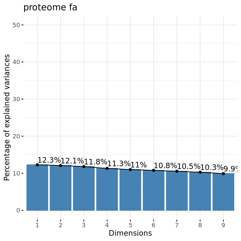
Negative control 2: eigen values of PCs from a data matrix with row-wise shuffled values.
#### Plot PC1 vs PC2 with condition-specific colors ####
fviz_pca_ind(xShuffledRowsPCA, axes = c(1,2),
             col.ind = metadata$condition,
             repel = TRUE # Avoid overlap between labels
)
Negative control 2: PC plots from a data matrix with row-wise shuffled values.
#### Plot PC4 vs PC3 with condition-specific colors ####
fviz_pca_ind(xShuffledRowsPCA, axes = c(3,4),
             col.ind = metadata$condition,
             repel = TRUE # Avoid overlap between labels
)
Negative control 2: PC plots from a data matrix with row-wise shuffled values.
#### Plot PC5 vs PC6 with condition-specific colors ####
fviz_pca_ind(xShuffledRowsPCA, axes = c(5, 6),
             col.ind = metadata$condition,
             repel = TRUE # Avoid overlap between labels
)
Negative control 2: PC plots from a data matrix with row-wise shuffled values.