DU-Bii Study cases - TCGA
DUBii 2019
Jacques van Helden
2019-02-16
## Define parameters for the analysis
parameters <- list(
  epsilon = 0.1,
  gene.filter.min.count = 10,
  gene.filter.percent.zeros = 95,
  gzip.output.files = TRUE,
  alpha = 0.01,
  p.adjust.method = "fdr"
)

kable(t(data.frame(parameters)), col.names = "Parameter value")| Parameter value | |
|---|---|
| epsilon | 0.1 |
| gene.filter.min.count | 10 |
| gene.filter.percent.zeros | 95 |
| gzip.output.files | TRUE |
| alpha | 0.01 |
| p.adjust.method | fdr |
Introduction
Data source
Recount2 (https://jhubiostatistics.shinyapps.io/recount/) is a database rasembling several thousands of human RNA-seq studies, that were all processed with a same workflow in order to ensure the consistency of the transcriptome measurements. Recount2 provides direct access to tables of raw counts per gene, exon or transcript.
Requirements
- Recount library: https://bioconductor.org/packages/release/bioc/html/recount.html
# Install BiocManager if required
if (!requireNamespace("BiocManager", quietly = TRUE))
    install.packages("BiocManager")

# Install recount if required
if (!require(recount)) {
  BiocManager::install("recount", version = "3.8")
  require(recount)
}

# BiocManager::valid()
Working directory
## Set the working directory
workdir <- "~/TCGA_import"
dir.create(workdir, recursive = TRUE, showWarnings = FALSE)
setwd(workdir)

## Select a TCGA project
selected.project <- "Breast Invasive Carcinoma"
project.acronym <- "BIC"
message("\tSelected TCGA project\t", selected.project, " (", project.acronym, ")")

export.dir <- file.path(workdir, "data", project.acronym)
message("\tExport directory\t", export.dir)
dir.create(export.dir, recursive = TRUE, showWarnings = FALSE)
The downloaded and processed data will be saved in a working directory named TCGA_import in the user home folder (``r workdir). If required this directory is created automatically.
Data source
## Download the TCGA data from Recount2 database

## Set the recoutnID (to "TCGA")
recountID <- "TCGA"

# Specify the download directory
download.dir <- file.path(workdir, "downloads", recountID)
dir.create(download.dir, recursive = TRUE, showWarnings = FALSE)


## Data types to download
#download.types <- c("phenotype", "counts-gene", "rse-gene")
download.types <- c("rse-gene") # the rse-gene object contains both expression and pheno tables
localFiles <- c()
for (type in download.types) {
  message("Recount data type: ", type)
  ## Get the URL of the recount file
  ## (its extension will depend on the data type)
  recountURL <- download_study(
    recountID,
    outdir = download.dir,
    type = type,
    download = FALSE)
  message("\trecountURLL: ", recountURL)

  ## Define the local file name
  localFile <- file.path(download.dir, basename(recountURL))
  message("\tlocalFile: ", localFile)

  ## Index local file for later use
  localFiles[type] <- localFile


  ## Download the data only if required
  if (!file.exists(localFile)) {
    message("\tDowloading ", type, " from ReCount for study ", recountID)
    url <- download_study(
      recountID,
      outdir = download.dir,
      type = type)
  } else {
    message("\tfile already there: ", localFile)

  }
}
## Download the gene-level RangedSummarizedExperiment data
# download_study(project = "TCGA", type = "counts-gene", outdir = download.dir)
We downloaded the following file types from Recount2: rse-gene.
Data loading
# ## Choose a way to load the data.
# ## either from the Rdata file or from the TSV files .
# loadRdata <- TRUE
#
#
# if (loadRdata) {
## Load the RData memory image provided by Recount2, whcih contains the count table + pheno table
message("Loading TCGA data from Recount")
load(localFiles["rse-gene"])


## Extract the pheno table from the rse-gene object
phenoTable <- colData(rse_gene) ## phenotype per run
project.name <- "Breast invasive carcinoma"
message("Identifying samples for project ", project.name)
project.samples <- phenoTable$gdc_cases.tissue_source_site.project == project.name
message("\tNumber of project samples: ", sum(project.samples))

## Select the columns relevant for the Breast cancer study
immuno.columns <- c(
  ER = "xml_breast_carcinoma_estrogen_receptor_status",
  PR = "xml_breast_carcinoma_progesterone_receptor_status",
  HER2 = "xml_lab_proc_her2_neu_immunohistochemistry_receptor_status")
message("Immuno marker columns:\n\t", paste(collapse = "\n\t", immuno.columns))

## Only keep project samples with valid markers (i.e. Negative or Positive), discard Undertermined, Equivocal and  NA
valid.markers <- c("Negative", "Positive")
message("Selecting samples with valid immuno markers: ", paste(collapse = ", ", valid.markers))
valid.samples <-
  project.samples &
  apply(is.na(phenoTable[, immuno.columns]), 1, sum) == 0 &
  phenoTable[, immuno.columns["ER"]] %in% valid.markers &
  phenoTable[, immuno.columns["PR"]] %in% valid.markers &
  phenoTable[, immuno.columns["HER2"]] %in% valid.markers
# table(valid.samples)
message("\tvalid samples: ", sum(valid.samples))

## Subset the expression data by selecting the valid samples
message("Extracting expression data for valid samples")
rse.valid.samples <- subset(rse_gene, select = valid.samples)
# dim(rse.valid.samples)

## Extract a pheno table for the subset
pheno <- colData(rse.valid.samples)
# dim(pheno.valid.samples)

## Scale counts by mapped reads, in order to to get read counts per gene
#rse.valid.samples.scaled <- scale_counts(rse.valid.samples, by = "mapped_reads")
# summary(assay(rse.valid.samples.scaled)[,1:7])
## WARNING: THIS DOES NOT WORK WITH THIS DATASET: ALL VALUES ARE SET TO 0.
## I THIS COMMENT IT

## Extract the count table from the rse-gene object
message("Extracting counts per gene")
counts.per.gene <- assay(rse.valid.samples)
# summary(counts.per.gene[, 1:10])
# dim(counts.per.gene)


# dim(phenoTable)
## NOTE: this phenoTable is a complex object: a DataFrame whose cells may be a list containing a table.
## To avoid messing around, I prefer to use the TSV version of the pheno table.
# dim(pheno)
# class(pheno)

#
#   # dim(countTable)
# } else {
#   ## Load the data from the TSV files downloaded from Recount2
#
#
#   ## Load the TCGA count table.
#   ## We use gzfile to directly load the zgipped file,
#   ## and data.table:::fread() to accelerate the reading.
#   ## system.time(counts.per.gene <- read.delim(file = gzfile(localFiles["counts-gene"]))) ## This takes 430 seconds
#   message("Loading counts per gene")
#   system.time(counts.per.gene <- fread(file = localFiles["counts-gene"]))
#   # This takes 29 seconds
#
#   ## Load the TCGA pheno table
#   message("Reading phenotype table")
#   pheno <- read.delim(file = localFiles["phenotype"])
#   # dim(pheno)
#
#   # dim(counts.per.gene)
# }


message("Selected dataset (project and valid markers)")
message("\tRead count table contains ", nrow(counts.per.gene), " rows (genes) x ", ncol(counts.per.gene), " columns (samples). ")
message("\tPheno table contains ", nrow(pheno), " rows (samples) x ", ncol(pheno), " columns (sample attributes). ")
The full TCGA gene count table contains 819 samples (columns) and 58037 genes (rows).
kable(sort(table(phenoTable$gdc_cases.project.name), decreasing = TRUE),
      caption = "Number of samples per TGCA project. ",
col.names = c("Project","samples"))| Project | samples |
|---|---|
| Breast Invasive Carcinoma | 1246 |
| Kidney Renal Clear Cell Carcinoma | 616 |
| Lung Adenocarcinoma | 601 |
| Uterine Corpus Endometrial Carcinoma | 589 |
| Thyroid Carcinoma | 572 |
| Prostate Adenocarcinoma | 558 |
| Lung Squamous Cell Carcinoma | 555 |
| Head and Neck Squamous Cell Carcinoma | 548 |
| Colon Adenocarcinoma | 546 |
| Brain Lower Grade Glioma | 532 |
| Skin Cutaneous Melanoma | 473 |
| Stomach Adenocarcinoma | 453 |
| Bladder Urothelial Carcinoma | 433 |
| Ovarian Serous Cystadenocarcinoma | 430 |
| Liver Hepatocellular Carcinoma | 424 |
| Kidney Renal Papillary Cell Carcinoma | 323 |
| Cervical Squamous Cell Carcinoma and Endocervical Adenocarcinoma | 309 |
| Sarcoma | 265 |
| Esophageal Carcinoma | 198 |
| Pheochromocytoma and Paraganglioma | 187 |
| Pancreatic Adenocarcinoma | 183 |
| Rectum Adenocarcinoma | 177 |
| Glioblastoma Multiforme | 175 |
| Testicular Germ Cell Tumors | 156 |
| Acute Myeloid Leukemia | 126 |
| Thymoma | 122 |
| Kidney Chromophobe | 91 |
| Mesothelioma | 87 |
| Uveal Melanoma | 80 |
| Adrenocortical Carcinoma | 79 |
| Uterine Carcinosarcoma | 57 |
| Lymphoid Neoplasm Diffuse Large B-cell Lymphoma | 48 |
| Cholangiocarcinoma | 45 |
For the study case, we select the project 1246, which contains 1246 samples.
Class labels
The class of cancer is defined by combining three immunological markers:
- HER2,
- ER (estrogen receptor)
- Pr (progesterone receptor)
The tables below provide summaries of the marker status for all samples.
project.markers <- phenoTable[project.samples, immuno.columns]
colnames(project.markers) <- names(immuno.columns)
summary(as.data.frame(project.markers))
ER PR HER2
: 0 : 0 : 0
Indeterminate: 3 Indeterminate: 5 Equivocal :201
Negative :273 Negative :387 Indeterminate: 12
Positive :910 Positive :793 Negative :636
NA's : 60 NA's : 61 Positive :190
NA's :207 Marker status summary after having discarded invalid values.
valid.markers <- phenoTable[valid.samples, immuno.columns]
colnames(valid.markers) <- names(immuno.columns)
summary(as.data.frame(valid.markers))
ER PR HER2
: 0 : 0 : 0
Indeterminate: 0 Indeterminate: 0 Equivocal : 0
Negative :184 Negative :267 Indeterminate: 0
Positive :635 Positive :552 Negative :631
Positive :188 We discard the samples for which any of the markers is undefined (NA), “Indeterminate” or “Equivocal”. In total, this leaves us with 819 samples.
We then assign a class label to each sample, indicating its cancer subtype, which is assigned based on the combination of the three immunological markers.
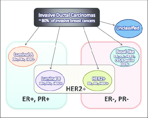
Figure 1. Definition of breast cancer subtypes based on immunological markers HER2, ER (Estrogen Receptor), and PR (Progesterone Receptor)
## Define sample classes based on the combination of 3 marker values
pheno$cancer.type <- rep("Unclassified", length.out = nrow(pheno))

luminal.A <-
  pheno[, immuno.columns["ER"]] == "Positive" &
  pheno[, immuno.columns["PR"]] == "Positive" &
  pheno[, immuno.columns["HER2"]] == "Negative"
pheno[luminal.A, "cancer.type"] <- "Luminal.A"

luminal.B <-
  pheno[, immuno.columns["ER"]] == "Positive" &
  pheno[, immuno.columns["PR"]] == "Positive" &
  pheno[, immuno.columns["HER2"]] == "Positive"
pheno[luminal.B, "cancer.type"] <- "Luminal.B"

her2plus <-
  pheno[, immuno.columns["ER"]] == "Negative" &
  pheno[, immuno.columns["PR"]] == "Negative" &
  pheno[, immuno.columns["HER2"]] == "Positive"
pheno[her2plus, "cancer.type"] <- "HER2pos"

basal.like <-
  pheno[, immuno.columns["ER"]] == "Negative" &
  pheno[, immuno.columns["PR"]] == "Negative" &
  pheno[, immuno.columns["HER2"]] == "Negative"
pheno[basal.like, "cancer.type"] <- "Basal.like"

kable(sort(decreasing = TRUE, table(pheno[, "cancer.type"])), useNA = "ifany", caption = "Number of samples per cancer subtype. Cancer subtypes were defined based on the combination of HER2, ER and PR markers. ")| Var1 | Freq |
|---|---|
| Luminal.A | 422 |
| Basal.like | 131 |
| Luminal.B | 118 |
| Unclassified | 107 |
| HER2pos | 41 |
## Get the identifiers of the selected samples
selected.sample.ids <- rownames(pheno)
# summary(selected.sample.ids %in% colnames(counts.per.gene))
# summary(colnames(counts.per.gene) %in% selected.sample.ids)

## Get the subset of the big count table corresponding to our selected IDs
## Note the special notation due to the specific class of the fread() result.
# if (!loadRdata) {
#   selected.counts <- as.data.frame(counts.per.gene[, ..selected.sample.ids])
# }
# dim(selected.counts)
# summary(selected.counts[, 1:10])
# summary(counts.per.gene[, 1:10])
Gene filtering
Percent zero counts
## Discard genes having zeros in at least 95% of samples
message("Applying threshold on the percent of non-zero counts per gene: ", parameters$gene.filter.percent.zeros, "%")
percent.zeros <- 100*apply(counts.per.gene == 0, 1, sum) / ncol(counts.per.gene)
hist(percent.zeros, breaks = 20, col = "#DDDDDD",
     main = "Filter on the percentage of zero counts",
     xlab = "Percent of samples", ylab = "Number of genes", las = 1)
arrows(x0 = parameters$gene.filter.percent.zeros,
       y0 = 10000,
       x1 = parameters$gene.filter.percent.zeros,
       y1 = 6000,
       col = "red", lwd = 2,
       angle = 30, length = 0.1)
text(x = parameters$gene.filter.percent.zeros,
     y = 10000,
     labels = paste(sep = "", parameters$gene.filter.percent.zeros, "%"),
     col = "red", pos = 3)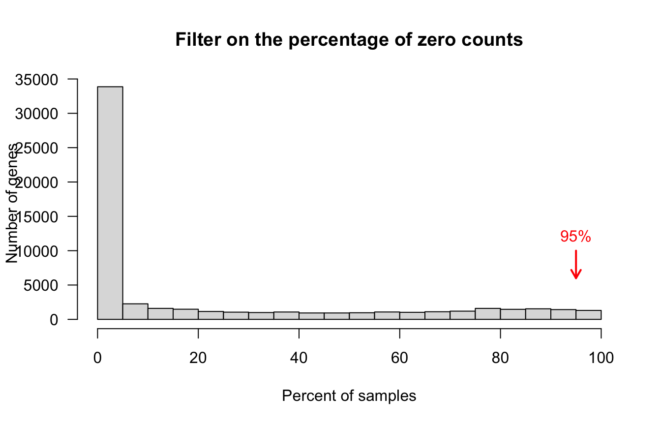
Frequency of samples with zero counts per gene. Genes exceeding the thresold (red arrow) were filtered out.
Min counts per gene
min.count <- apply(counts.per.gene, 1, min)
summary(min.count)
Min. 1st Qu. Median Mean 3rd Qu. Max.
0 0 0 6824 938 2168821 hist(log2(min.count + parameters$epsilon), breaks = 100, col = "#BBBBFF",
xlab = "log2(min count per gene)",
ylab = "Number of genes", las = 1,
main = "Filtering on min count per gene")
arrows(x0 = log2(parameters$gene.filter.min.count),
y0 = 3000,
x1 = log2(parameters$gene.filter.min.count),
y1 = 1000,
col = "red", lwd = 2,
angle = 30, length = 0.1)
text(x = log2(parameters$gene.filter.min.count),
y = 3000,
labels = paste(sep = "", "log2(",
parameters$gene.filter.min.count,
") = ", signif(digits = 3, log2(parameters$gene.filter.min.count))),
col = "red", pos = 3)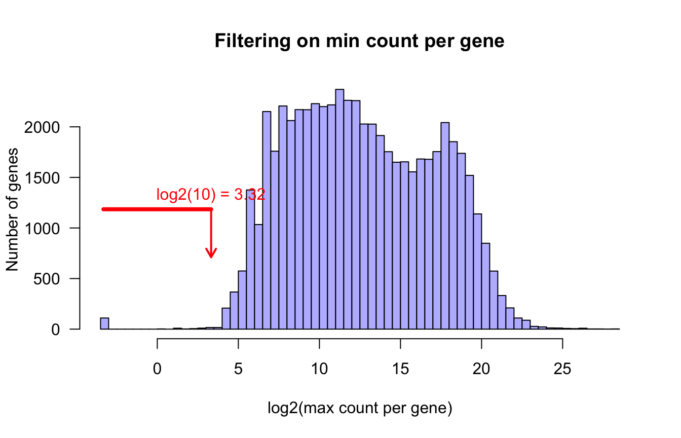
Distribution of min counts per gene. Genes below the thresold (red arrow) are filtered out.
filtered.out.genes <-
  percent.zeros > parameters$gene.filter.percent.zeros |
  min.count < parameters$gene.filter.min.count
# table(kept.genes)

## Genes passing the filters
filtered.genes <- !filtered.out.genes
filtered.counts <- counts.per.gene[filtered.genes, ]
We discard “undetected” genes, i.e. those having zero counts in at least 95 percent of the samples, or those with a maximal count inferior to 10. This led us to discard 37788 genes.
Differential expression
We select differentially expressed genes in order to produce a file with a restricted number of genes for clustering.
## Use the DESeqDataSetFromMatrix to create a DESeqDataSet object
message("Creating DESeq2 dataset")
dds0 <- DESeqDataSetFromMatrix(
  countData = as.data.frame(filtered.counts),
  colData = data.frame(cancer.type = as.factor(pheno[, "cancer.type"])),
  design = ~ cancer.type)

# print(dds0) # Have a look at the short description of the DESeqDataSet

## PROBLEM: the differential analysis with DESeq2 is stuck.
#@ Probably because there are too many samples ?
## TO DO:
## - test it on IFB cluster
## - test edgeR as selection method
## - select a random subset of the samples

# ## Run  differential expression analysis with DESeq2
# message("Running differential expression analysis with DESeq2")
# dds0 <- DESeq(dds0)
#
# # Cast the results from DESeq differential expression analysis
# DEGtable <- results(dds0, independentFiltering = FALSE)
## Detection of Differentially Expressed Genes (DEG) with edgeR
message("Detecting Differentially Expressed Genes (DEG) with edgeR")
## Build a "model matrix" from the class labels
## This matrix contains one row per sample and one column per class
designMat <- model.matrix(~ pheno$cancer.type)
# View(designMat)
## Build an edgeR::DGEList object which is required to run edgeR DE analysis
dgList <- DGEList(counts = filtered.counts)
# class(dgList)
# is(dgList)
## Estimate the dispersion parameters.
message("\tedgeR\tEstimating dispersion")
dgList <- estimateDisp(dgList, design = designMat)
## Fit edgeR model for differential expression analysis.
## We chose glmQLFit because it is claimed to offer a more accurate control of type I error.
message("\tedgeR\tmodel fitting with glmQLFit()")
fit <- glmQLFit(dgList, design = designMat)
## Run test to detect differentially expressed genes
message("\tedgeR\tdetecting differentially expressed genes with glmQLFTest()")
qlf <- glmQLFTest(fit, coef = 2:ncol(designMat))
message("\tedgeR\t")
qlf.TT <- topTags(qlf, n = nrow(qlf$table), sort.by = "none",
adjust.method = parameters$p.adjust.method)
# class(qlf.TT)
# Note: the adusted p-values are co-linear with the nominal p-value,
## which is not supposed to be the case with BH correction.
## I should test this.
# plot(qlf.TT$table$PValue, qlf.TT$table$FDR, log = "xy", col = "grey")
## Select differentially expressed genes
edgeR.DEG.table <- qlf.TT$table
DEG <- edgeR.DEG.table$FDR < parameters$alpha
# sum(DEG)
## Awful: almost all genes are declared positive
## The p-value histogram shows indeed that almost no gene has
## a nominal pvalue > 0.5 (typical lambda for Storey-Tibshirani 2003).
hist(edgeR.DEG.table$PValue, breaks = 20, col = "grey")
Normalization of the counts per gene
We use DESeq2 function estimateSizeFactors() to estimate the library-wise size factors, which will be used to standardize the counts.
We then apply a log2 transformation in order to normalize these standardized counts.
## Normalizing using the method for an object of class"CountDataSet"
message("Normalizing count with DESeq2")
dds.norm <-  estimateSizeFactors(dds0)
# sizeFactors(dds.norm)

counts.norm <- counts(dds.norm) + parameters$epsilon
# dim(counts.norm)
counts.log2.norm <- log2(counts.norm)
# dim(counts.log2.norm)
log2.count.breaks <- seq(
from = log2(parameters$epsilon),
to = 32,
by = 0.4)
par(mfrow = c(2, 1))
hist(unlist(log2(unlist(counts.per.gene + parameters$epsilon))), main = "Log2(raw counts)",
xlab = "log2(raw counts + epsilon)",
ylab = "Number of measures",
breaks = log2.count.breaks,
col = "#FFDDBB")
hist(unlist(counts.log2.norm), main = "Normalized counts",
xlab = "log2(standardized counts)",
ylab = "Number of measures",
breaks = log2.count.breaks,
col = "#DDFFBB")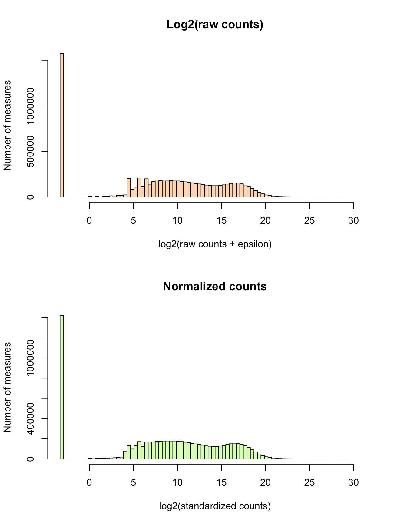
Histogram of all counts. (a) Before filtering and standardization. Distribution of log2(raw counts + epsilon). The epsilon is added to avoid -Inf values for log2-transformed zeros. (b) Normalised counts. Normalization consists in scaling counts in order to ensure library size standardization, followed by a log2 transformation.
par(mfrow = c(1, 1))Exported tables
The selected counts per gene and pheno table were exported in tab-separated value (TSV) format.
pheno.export.columns <- names(pheno)
for (col in pheno.export.columns) {
  ## Discard columns containing only NA values
  nona <- sum(!is.na(pheno[, col]))
  if (nona == 0) {
    # message("\tDiscarding NA-only pheno column\t", col, "\tnoNA = ", nona)
    pheno.export.columns <- setdiff(pheno.export.columns, col)
  }

  # Discard columns containing muli-value lists
  if (class(pheno[, col]) == "list") {
    message("\tDiscarding list-type pheno column\t", col)
    pheno.export.columns <- setdiff(pheno.export.columns, col)

  }
}
message("Exporting ", length(pheno.export.columns), " pheno columns among ", ncol(pheno))

## Export the non-problematic columns of the pheno table
pheno.file <- paste(sep = "", project.acronym, "_pheno.tsv.gz")
pheno.path <- file.path(export.dir, pheno.file)
if (parameters$gzip.output.files) {
  pheno.path <- gzfile(pheno.path, "w") ## Compress file
}
write.table(x = as.data.frame(pheno[, pheno.export.columns]),
            file = pheno.path,
            sep = "\t", quote = FALSE, row.names = FALSE)
if (parameters$gzip.output.files) {
  close(pheno.path)
}

## Export a small subset of relevant fields from the pheno table
pheno.selected.columns <- c(
  "cancer.type",
  immuno.columns
)
sample.class.file <- paste(sep = "", project.acronym, "_sample-classes.tsv.gz")
sample.class.path <- file.path(export.dir, sample.class.file)
if (parameters$gzip.output.files) {
  sample.class.path <- gzfile(sample.class.path, "w") ## Compress file
}
write.table(x = as.data.frame(pheno[, pheno.selected.columns]),
            file = sample.class.path,
            sep = "\t", quote = FALSE, row.names = FALSE)
if (parameters$gzip.output.files) {
  close(sample.class.path)
}


## Export counts per gene
count.file <- paste(sep = "", project.acronym, "_counts_all-genes.tsv")
count.path <- file.path(export.dir, count.file)
if (parameters$gzip.output.files) {
  count.path <- gzfile(count.path, "w") ## Compress file
}
write.table(x = counts.per.gene,
            file = count.path,
            sep = "\t", quote = FALSE, row.names = TRUE, col.names = NA)
if (parameters$gzip.output.files) {
  close(count.path)
}

## Export raw counts
filtered.count.file <- paste(sep = "", project.acronym, "_counts_filtered-genes.tsv")
filtered.count.path <- file.path(export.dir, filtered.count.file)
if (parameters$gzip.output.files) {
  filtered.count.path <- gzfile(filtered.count.path, "w") ## Compress file
}
write.table(x = filtered.counts,
            file = filtered.count.path,
            sep = "\t", quote = FALSE, row.names = TRUE, col.names = NA)
if (parameters$gzip.output.files) {
  close(filtered.count.path)
}

# list.files(export.dir)

## Export normalized counts
norm.count.file <- paste(sep = "", project.acronym, "_log2-norm-counts_all-genes.tsv")
norm.count.path <- file.path(export.dir, norm.count.file)
if (parameters$gzip.output.files) {
  norm.count.path <- gzfile(norm.count.path, "w") ## Compress file
}
write.table(x = counts.log2.norm,
            file = norm.count.path,
            sep = "\t", quote = FALSE, row.names = TRUE, col.names = NA)
if (parameters$gzip.output.files) {
  close(norm.count.path)
}

## Export normalized counts
filtered.norm.count.file <- paste(sep = "", project.acronym, "_log2-norm-counts_filtered-genes.tsv")
filtered.norm.count.path <- file.path(export.dir, filtered.norm.count.file)
if (parameters$gzip.output.files) {
  filtered.norm.count.path <- gzfile(filtered.norm.count.path, "w") ## Compress file
}
# dim(counts.log2.norm)
write.table(x = counts.log2.norm,
            file = filtered.norm.count.path,
            sep = "\t", quote = FALSE, row.names = TRUE, col.names = NA)
if (parameters$gzip.output.files) {
  close(filtered.norm.count.path)
}

## Export normalized counts for DEG only
DEG.norm.count.file <- paste(sep = "", project.acronym, "_log2-norm-counts_DEG_", parameters$p.adjust.method, "_", parameters$alpha, ".tsv")
DEG.norm.count.path <- file.path(export.dir, DEG.norm.count.file)
if (parameters$gzip.output.files) {
  DEG.norm.count.path <- gzfile(DEG.norm.count.path, "w") ## Compress file
}
# dim(counts.log2.norm)
write.table(x = counts.log2.norm[DEG, ],
            file = DEG.norm.count.path,
            sep = "\t", quote = FALSE, row.names = TRUE, col.names = NA)
if (parameters$gzip.output.files) {
  close(DEG.norm.count.path)
}| Contants | File name |
|---|---|
| Export directory | ~/TCGA_import/data/BIC |
| Pheno table | ~/TCGA_import/data/BIC |
| Counts per gene (all genes) | BIC_counts_all-genes.tsv |
| Counts per gene (filtered genes) | BIC_counts_filtered-genes.tsv |
| Normalized counts per gene (all genes) | BIC_log2-norm-counts_all-genes.tsv |
| Normalized counts per gene (filtered genes) | BIC_log2-norm-counts_filtered-genes.tsv |
| Normalized counts per gene (differentially expressed genes) | BIC_log2-norm-counts_DEG_fdr_0.01.tsv |
Contact: Jacques.van-Helden@univ-amu.fr