Tutorial: exploration of multi-omics data

DUBii 2021

Goals of this tutorial

This tutorial aims at

1. Learn to load files from remote locations, either directly or by downloading them to a local folder.

2. Apply some of the methods taught in the previous courses in order to explore a data set.

3. Show some convenient ways of combinig R code and markdown elements within an R markdown document in order to obtain a well-formatted scientific report.

   • configuring the parameters in the yaml header of the R markdown file
   • organising the code in R chunks
   • writing, documenting and using an R function
   • generating an ugly figure, improving it and controlling its incorporation in the report (size, legend)

Study case : mouse kidney

As study case for this tutorial, we will use multi-omics data from a study published by Pavkovic et al. (2019), which combines transctiptomics (RNA-seq) and proteomics approaches to understand the molecular mechanisms underlying the kidney fibrosis pathology.

The authors applied two commonly used treatments to induce kidney fibrosis in mouse:

• a reversible chemical-induced injury model, denoted as FA for folic acid induced nephropathy;

• an irreversible surgically-induced fibrosis model, denoted as UUO for unilateral uretral obstruction.

References and data sources

• Reference: Pavkovic, M., Pantano, L., Gerlach, C.V. et al. Multi omics analysis of fibrotic kidneys in two mouse models. Sci Data 6, 92 (2019) https://doi.org/10.1038/s41597-019-0095-5

• Mouse fibrotic kidney browser: http://hbcreports.med.harvard.edu/fmm/

• Data on Zenodo: https://zenodo.org/record/2592516

Data preparation

A description of the study case can be found in the Mus musculus section of the the DUBii study cases repository repository.

We also provide there a detailed explanation of the data preparation steps:

• downloading the data from its original source repository,
• exploring the datasets it with various graphical representtions,
• computing some descriptive statistics on the different samples,
• pre-processing,
• storing the results in a memory image.

Data file naming

We prepared the data from Pavkovic as a text file with tab-separated values (tsv files).

All the files are available on github: - https://github.com/DU-Bii/module-3-Stat-R/tree/master/stat-R_2021/data/pavkovic_2019

The files are named according to the following convention:

• the prefix indicate the data type

  • fa: folic acid induced nephropathy (reversible), transcriptome data
  • pfa: folic acid induced nephropathy, proteome data
  • uuo: unilateral uretral obstruction (irreversible), transcriptome data
  • puuo: unilateral uretral obstruction, proteome data

• The suffix indicates the data normalisation

  • raw: transcriptome counts provided by the authors (note: not integer, because their raw data was already somehow normalized)
  • normalized¨: transcriptome counts standardized to achieve the same third quartile for each sample
  • log2: log2 transformation for proteome data

• the metadata files contain a short description of each sample (one row per sample). Note that the last column contains a sample-specific color specification in hexadecimal web color code to facilitate the drawings. Don’t hesitate to chose other colors according to your personal taste.

R style

The R code belows follows the tidyverse styling guide (https://style.tidyverse.org/).

Approach for this tutorial

This tutorial will consist of exercises that can be realised in a stepwise way, with alternance of working sessions and live demos of the solutions, in order to make sure that all the trainees acquire each step.

Data exploration

Before computing any descriptive parameter on a dataset, I generallyi attempt to get a picture of the whole distribution.

Finding a data file on github

We will provide here a magic recipe to download the data from the github repository to your local folder, and to load it in R.

## specify the base URL from which data files can be downloaded 
url_base <- "https://github.com/DU-Bii/module-3-Stat-R/raw/master/stat-R_2021/data/pavkovic_2019"


## Choose a specific data file
data_prefix <- "pfa" ## proteome data of folic-acid treated mouse
data_suffix <- "model" ## no normalization
file_name <- paste0(data_prefix, "_", data_suffix, "_counts.tsv.gz")

## Compose the URL to download the file from github
url <- file.path(url_base, file_name)

message("URL: ",  url)

Loading a data file directly from github

Now we defined the URL, we can easily load the file directly from github to a data frame in our R environement.

## this requires to load a specific package
if (!require("data.table")) {
  install.packages("data.table")
}
library(data.table)

pfa <- fread(url, header = TRUE, sep = "\t")
dim(pfa)
names(pfa)
kable(head(pfa))

Downloading a data file and storing it locally once forever

We can now download the data file to a local folder, but we would like to do this only once.

## Specify the path relative to your home directory (~)
local_folder <- "~/DUBii-m3_data/pavkovic_2019"
local_file <- file.path(local_folder, file_name)

## Create the local data folder if it does not exist
dir.create(local_folder, showWarnings = FALSE, recursive = TRUE)

## Download the file ONLY if it is not already there
if (!file.exists(local_file)) {
  message("Downloading file from github to local file\n\t", 
          local_file)
  download.file(url = url, destfile = local_file)
} else {
  message("Local file already exists, no need to download\n\t", 
          local_file)
}

Loading the local copy of your data file

We will now load the proteome file, with the following parameters

• the first row contains the column headers
• the first columnt contains the protein IDs, and we would like to have them as row.names for the loaded data frame. This is a bit tricky because some protein names are diplicated. We use the very convenient function make.names(x, unique = TRUE).

## Load the data from the local file
pfa <- read.delim(file = local_file, header = TRUE, sep = "\t")

kable(head(pfa), caption = "Data frame just after loading")

Data frame just after loading

id	normal_1	normal_2	day1_1	day1_2	day2_1	day2_2	day7_1	day7_2	day14_1	day14_2
ENSMUSG00000037686	531.2680	651.7200	335.5910	334.8460	197.1740	307.194	123.2060	272.6190	93.7247	196.1590
ENSMUSG00000027831	221.6020	266.3590	175.4090	159.4190	234.8080	256.927	149.9380	315.0590	110.5880	126.3600
ENSMUSG00000039201	26.0723	29.1331	57.7329	45.8475	81.6009	88.870	29.8560	44.5586	13.6292	27.6568
ENSMUSG00000031095	4363.0500	4784.0800	4064.4800	3917.2900	4599.0300	5957.030	2806.5200	6792.0900	2022.5100	3226.7500
ENSMUSG00000034931	879.2790	1065.3900	914.2870	928.2760	1000.1000	1264.270	738.3520	1362.0700	466.4440	714.5870
ENSMUSG00000038208	68.2225	89.8871	57.9041	76.3510	84.8474	105.245	72.8696	138.9810	40.8101	59.2117

## Convert the first colum to row names
row.names(pfa) <- make.names(as.vector(pfa$id), unique = TRUE)
pfa <- pfa[, -1] ## Suppress the ID colimn
kable(head(pfa), caption = "Data frame with row names")

Data frame with row names

	normal_1	normal_2	day1_1	day1_2	day2_1	day2_2	day7_1	day7_2	day14_1	day14_2
ENSMUSG00000037686	531.2680	651.7200	335.5910	334.8460	197.1740	307.194	123.2060	272.6190	93.7247	196.1590
ENSMUSG00000027831	221.6020	266.3590	175.4090	159.4190	234.8080	256.927	149.9380	315.0590	110.5880	126.3600
ENSMUSG00000039201	26.0723	29.1331	57.7329	45.8475	81.6009	88.870	29.8560	44.5586	13.6292	27.6568
ENSMUSG00000031095	4363.0500	4784.0800	4064.4800	3917.2900	4599.0300	5957.030	2806.5200	6792.0900	2022.5100	3226.7500
ENSMUSG00000034931	879.2790	1065.3900	914.2870	928.2760	1000.1000	1264.270	738.3520	1362.0700	466.4440	714.5870
ENSMUSG00000038208	68.2225	89.8871	57.9041	76.3510	84.8474	105.245	72.8696	138.9810	40.8101	59.2117

Writing a function to download a file only once

Write a functions that will download a file from a remote location to a local folder, but do this only if the local file is not yet present there.

Note that we use the roxygen2 format to write the documentation of this function. In any programming language, a function should always be documented in order to enable other people to use it, and the doc is also very useful for a developer to reuse her/his own code. The documentation becomes particularly interesting when you start building your own R packages, since it will automatically generate the help pages.

The documentation of a function should include - a description of what it does - the author name and a way to contact her/him - a description of each parameter (argument) of the function - a description of the return value

Roxygen2 provides is a very convenient way of documenting a function, because - the formalism is very simple - the doc comes together with the code of the function (by default, R functions are documented in a separate file)

#' @title Download a file only if it is not yet here
#' @author Jacques van Helden email{Jacques.van-Helden@@france-bioinformatique.fr}
#' @param url_base base of the URL, that will be prepended to the file name
#' @param file_name name of the file (should not contain any path)
#' @param local_folder path of a local folder where the file should be stored
#' @return the function returns the path of the local file, built from local_folder and file_name
#' @export
download_only_once <- function(url_base, 
                             file_name,
                             local_folder) {

  ## Define the source URL  
  url <- file.path(url_base, file_name)
  message("Source URL\n\t",  url)

  ## Define the local file
  local_file <- file.path(local_folder, file_name)
  
  ## Create the local data folder if it does not exist
  dir.create(local_folder, showWarnings = FALSE, recursive = TRUE)
  
  ## Download the file ONLY if it is not already there
  if (!file.exists(local_file)) {
    message("Downloading file from source URL to local file\n\t", 
            local_file)
    download.file(url = url, destfile = local_file)
  } else {
    message("Local file already exists, no need to download\n\t", 
            local_file)
  }
  
  return(local_file)
}

We can now use our new function download_only_once() to download the files from the folic acid dataset and store them in a local folder. We will download successively :

• transcriptome data (fa)
• transcriptome medata
• proteome data (pfa)
• proteome medata

## Specify the basic parameters
pavkovic_base <- "https://github.com/DU-Bii/module-3-Stat-R/raw/master/stat-R_2021/data/pavkovic_2019"
pavkovic_folder <- "~/DUBii-m3_data/pavkovic_2019"

#### Dowload folic acid data and metadata ####

## Transcriptome data table
local_fa_file <- download_only_once(
  url_base = pavkovic_base, 
  file_name = "fa_raw_counts.tsv.gz",
  local_folder =  pavkovic_folder
)

## Normalised transcriptome data table
local_fa_norm_file <- download_only_once(
  url_base = pavkovic_base, 
  file_name = "fa_normalized_counts.tsv.gz",
  local_folder =  pavkovic_folder
)


## Transcriptome metadata
fa_metadata_file <- download_only_once(
  url_base = pavkovic_base, 
  file_name = "fa_transcriptome_metadata.tsv",
  local_folder =  pavkovic_folder
)

## FA proteome data table
local_pfa_file <- download_only_once(
  url_base = pavkovic_base, 
  file_name = "pfa_model_counts.tsv.gz",
  local_folder =  pavkovic_folder
)

## FA proteome metadata
pfa_metadata_file <- download_only_once(
  url_base = pavkovic_base, 
  file_name = "pfa_proteome_metadata.tsv",
  local_folder =  pavkovic_folder
)


## UUO proteome data table
local_puuo_file <- download_only_once(
  url_base = pavkovic_base, 
  file_name = "puuo_model_counts.tsv.gz",
  local_folder =  pavkovic_folder
)

After having run the chunk of code above, try to re-run it. In principle, you should just receive messages telling you that the files are already there.

Loading the files

We now write a function load_fix_row_names() that loads a data file and takes a specified column as row names, whilst automatically fixing potential problems due to duplicate labels in this column.

#' @title Load a tab-separated value file and manually set row ames after having forced them to unique values
#' @author Jacques van Helden email{Jacques.van-Helden@@france-bioinformatique.fr}
#' @param file file path
#' @param header=1 Header is set to 1 by default
#' @param sep="\t" Column separator is set to tab by default
#' @param rownames.col=1 Column containing the row names
#' @param ... all other parameters are passed to read.delim()
#' @return a data frame with the loaded data
load_fix_row_names <- function(file, 
                       header = 1, 
                       sep = "\t",
                       rownames.col = 1, 
                       ...) {
  x <- read.delim(file = file, ...)
  rownames(x) <- make.names(x[, rownames.col], unique = TRUE)
  x <- x[, -rownames.col]
  return(x)
}

We can now load the data from our local folder.

## Load transcriptome data (raw counts)
fa_by_read_delim <- read.delim(file = local_fa_file, sep = "\t", header = TRUE)

## Check the first lines of the loaded file
# dim(fa)
message("Loaded raw counts of FA transcriptome raw counts with read_delim(): ", 
        nrow(fa_by_read_delim), " rows x ", ncol(fa_by_read_delim), " columns")
kable(head(fa_by_read_delim), caption = "FA transcriptome loaded with read.delim()")

FA transcriptome loaded with read.delim()

rowname	day1_1	day1_2	day1_3	day14_1	day14_2	day14_3	day2_1	day2_2	day2_3	day3_1	day3_2	day3_3	day7_1	day7_2	day7_3	normal_1	normal_2	normal_3
ENSMUSG00000000001	2278.80022	1786.498848	2368.618959	627.758017	559.156031	611.4338605	2145.223456	262.454849	745.843632	987.1850529	1077.645231	1335.116771	1096.075988	1035.8458456	1090.0375905	483.2298191	1842.14841	475.696800
ENSMUSG00000000003	0.00000	0.000000	0.000000	0.000000	0.000000	0.0000000	0.000000	0.000000	0.000000	0.0000000	0.000000	0.000000	0.000000	0.0000000	0.0000000	0.0000000	0.00000	0.000000
ENSMUSG00000000028	36.27547	22.147861	39.484949	14.470759	10.167813	31.6910193	300.558779	4.771672	123.896184	51.8555945	8.434511	69.936866	6.665195	6.9552273	42.5783251	7.3515305	11.19676	1.034465
ENSMUSG00000000031	13.18853	7.151932	1.115304	0.867429	0.000000	0.0000000	1.711944	0.000000	5.260747	0.8022308	0.000000	0.000000	0.000000	0.8489214	1.7106814	0.8603067	0.00000	0.000000
ENSMUSG00000000037	0.00000	27.903213	6.897842	5.692254	1.901719	0.6549762	57.382077	0.000000	38.898261	8.9308534	6.966606	0.000000	7.939323	101.6481244	0.6500858	32.0575944	10.42322	0.000000
ENSMUSG00000000049	30.86001	4.861367	51.466810	26.152649	1.968290	55.8319868	10.796186	2.747397	1.805883	0.9468345	26.954566	7.666032	32.235700	6.7001171	33.9132330	27.7647071	38.42445	15.903837

## Load the same data with load_fix_row_names
fa <- load_fix_row_names(file = local_fa_file, rownames.col = 1)
message("Loaded raw counts of FA transcriptome raw counts with load_fix_row_names(): ", 
        nrow(fa), " rows x ", ncol(fa), " columns")
kable(head(fa), caption = "FA transcriptome loaded with load_fix_row_names()")

FA transcriptome loaded with load_fix_row_names()

	day1_1	day1_2	day1_3	day14_1	day14_2	day14_3	day2_1	day2_2	day2_3	day3_1	day3_2	day3_3	day7_1	day7_2	day7_3	normal_1	normal_2	normal_3
ENSMUSG00000000001	2278.80022	1786.498848	2368.618959	627.758017	559.156031	611.4338605	2145.223456	262.454849	745.843632	987.1850529	1077.645231	1335.116771	1096.075988	1035.8458456	1090.0375905	483.2298191	1842.14841	475.696800
ENSMUSG00000000003	0.00000	0.000000	0.000000	0.000000	0.000000	0.0000000	0.000000	0.000000	0.000000	0.0000000	0.000000	0.000000	0.000000	0.0000000	0.0000000	0.0000000	0.00000	0.000000
ENSMUSG00000000028	36.27547	22.147861	39.484949	14.470759	10.167813	31.6910193	300.558779	4.771672	123.896184	51.8555945	8.434511	69.936866	6.665195	6.9552273	42.5783251	7.3515305	11.19676	1.034465
ENSMUSG00000000031	13.18853	7.151932	1.115304	0.867429	0.000000	0.0000000	1.711944	0.000000	5.260747	0.8022308	0.000000	0.000000	0.000000	0.8489214	1.7106814	0.8603067	0.00000	0.000000
ENSMUSG00000000037	0.00000	27.903213	6.897842	5.692254	1.901719	0.6549762	57.382077	0.000000	38.898261	8.9308534	6.966606	0.000000	7.939323	101.6481244	0.6500858	32.0575944	10.42322	0.000000
ENSMUSG00000000049	30.86001	4.861367	51.466810	26.152649	1.968290	55.8319868	10.796186	2.747397	1.805883	0.9468345	26.954566	7.666032	32.235700	6.7001171	33.9132330	27.7647071	38.42445	15.903837

# hist(unlist(fa), breaks = 100)

## Load normalised data with load_fix_row_names
fa_norm <- load_fix_row_names(file = local_fa_norm_file, rownames.col = 1)
message("Loaded raw counts of FA transcriptome normalised counts with load_fix_row_names(): ", 
        nrow(fa_norm), " rows x ", ncol(fa_norm), " columns")
# dim(fa_norm)
kable(head(fa_norm), caption = "First lines of the loaded normalised counts of FA transcriptome with load_fix_row_names()")

First lines of the loaded normalised counts of FA transcriptome with load_fix_row_names()

	day1_1	day1_2	day1_3	day14_1	day14_2	day14_3	day2_1	day2_2	day2_3	day3_1	day3_2	day3_3	day7_1	day7_2	day7_3	normal_1	normal_2	normal_3
ENSMUSG00000000001	2711.22417	1094.745589	1331.5880610	728.668808	603.846446	646.124076	1185.658698	1239.4695	829.596362	928.1069573	1110.908359	951.071644	953.722863	1008.0265279	1001.4667413	719.032852	1247.299971	809.375515
ENSMUSG00000000003	0.00000	0.000000	0.0000000	0.000000	0.000000	0.000000	0.000000	0.0000	0.000000	0.0000000	0.000000	0.000000	0.000000	0.0000000	0.0000000	0.000000	0.000000	0.000000
ENSMUSG00000000028	42.82759	13.485108	21.9214582	16.244209	10.802262	33.839559	166.379146	23.6540	137.895374	48.8972257	8.244218	49.868925	6.091296	6.8109901	39.5074036	10.420766	7.448588	1.700369
ENSMUSG00000000031	15.46552	4.290716	0.5620887	1.160301	0.000000	0.000000	1.105509	0.0000	5.560297	0.9403313	0.000000	0.000000	0.000000	0.9729986	1.8375537	1.488681	0.000000	0.000000
ENSMUSG00000000037	0.00000	17.162865	3.9346207	6.961804	2.160452	1.057486	31.507014	0.0000	43.370319	8.4629814	7.213691	0.000000	6.961481	99.2458551	0.9187768	47.637787	6.771444	0.000000
ENSMUSG00000000049	36.87931	3.064797	28.6665222	30.167817	2.160452	59.219228	6.080301	14.1924	2.224119	0.9403313	27.824235	5.699306	27.845923	6.8109901	31.2384121	41.683064	25.731487	27.205900

## Load FA proteome data
pfa <- load_fix_row_names(file = local_pfa_file, rownames.col = 1)
message("Loaded raw counts of FA proteome (pfa)  with load_fix_row_names(): ", 
        nrow(pfa), " rows x ", ncol(pfa), " columns")
# dim(pfa)

## Load UUO proteome data
puuo <- load_fix_row_names(file = local_puuo_file, rownames.col = 1)
message("Loaded raw counts of UUO proteome (puuo)  with load_fix_row_names(): ", 
        nrow(puuo), " rows x ", ncol(puuo), " columns")
# dim(pfa)

## Check the first lines of the loaded file
kable(head(pfa), caption = "First lines of the proteome table")

First lines of the proteome table

	normal_1	normal_2	day1_1	day1_2	day2_1	day2_2	day7_1	day7_2	day14_1	day14_2
ENSMUSG00000037686	531.2680	651.7200	335.5910	334.8460	197.1740	307.194	123.2060	272.6190	93.7247	196.1590
ENSMUSG00000027831	221.6020	266.3590	175.4090	159.4190	234.8080	256.927	149.9380	315.0590	110.5880	126.3600
ENSMUSG00000039201	26.0723	29.1331	57.7329	45.8475	81.6009	88.870	29.8560	44.5586	13.6292	27.6568
ENSMUSG00000031095	4363.0500	4784.0800	4064.4800	3917.2900	4599.0300	5957.030	2806.5200	6792.0900	2022.5100	3226.7500
ENSMUSG00000034931	879.2790	1065.3900	914.2870	928.2760	1000.1000	1264.270	738.3520	1362.0700	466.4440	714.5870
ENSMUSG00000038208	68.2225	89.8871	57.9041	76.3510	84.8474	105.245	72.8696	138.9810	40.8101	59.2117

## Load proteome metadata
pfa_metadata <- read.delim(file = pfa_metadata_file, sep = "\t", header = TRUE)
kable(pfa_metadata, caption = "Metadata for the FA proteome dataset")

Metadata for the FA proteome dataset

dataType	sampleName	condition	sampleNumber	color
proteome	normal_1	normal	1	#BBFFBB
proteome	normal_2	normal	2	#BBFFBB
proteome	day1_1	day1	1	#FFFFDD
proteome	day1_2	day1	2	#FFFFDD
proteome	day2_1	day2	1	#BBD7FF
proteome	day2_2	day2	1	#BBD7FF
proteome	day7_1	day7	1	#FFDD88
proteome	day7_2	day7	2	#FFDD88
proteome	day14_1	day14	1	#FF4400
proteome	day14_2	day14	2	#FF4400

## Load transcriptome metadata
fa_metadata <- read.delim(file = fa_metadata_file, sep = "\t", header = TRUE)
kable(fa_metadata, caption = "Metadata for the transcriptome dataset")

Metadata for the transcriptome dataset

dataType	sampleName	condition	sampleNumber	color
transcriptome	day14_1	day14	1	#FF4400
transcriptome	day14_2	day14	2	#FF4400
transcriptome	day14_3	day14	3	#FF4400
transcriptome	day1_1	day1	1	#BBD7FF
transcriptome	day1_2	day1	2	#BBD7FF
transcriptome	day1_3	day1	3	#BBD7FF
transcriptome	day2_1	day2	1	#F0BBFF
transcriptome	day2_2	day2	2	#F0BBFF
transcriptome	day2_3	day2	3	#F0BBFF
transcriptome	day3_1	day3	1	#FFFFDD
transcriptome	day3_2	day3	2	#FFFFDD
transcriptome	day3_3	day3	3	#FFFFDD
transcriptome	day7_1	day7	1	#FFDD88
transcriptome	day7_2	day7	2	#FFDD88
transcriptome	day7_3	day7	3	#FFDD88
transcriptome	normal_1	normal	1	#BBFFBB
transcriptome	normal_2	normal	2	#BBFFBB
transcriptome	normal_3	normal	3	#BBFFBB

We can now use this function to download and load the different data files.

Graphical exploration of the data

Histogram

Draw histograms of the transcriptome and proteom data, all samples together.

pfa_vector <- unlist(as.vector(pfa))
hist(pfa_vector)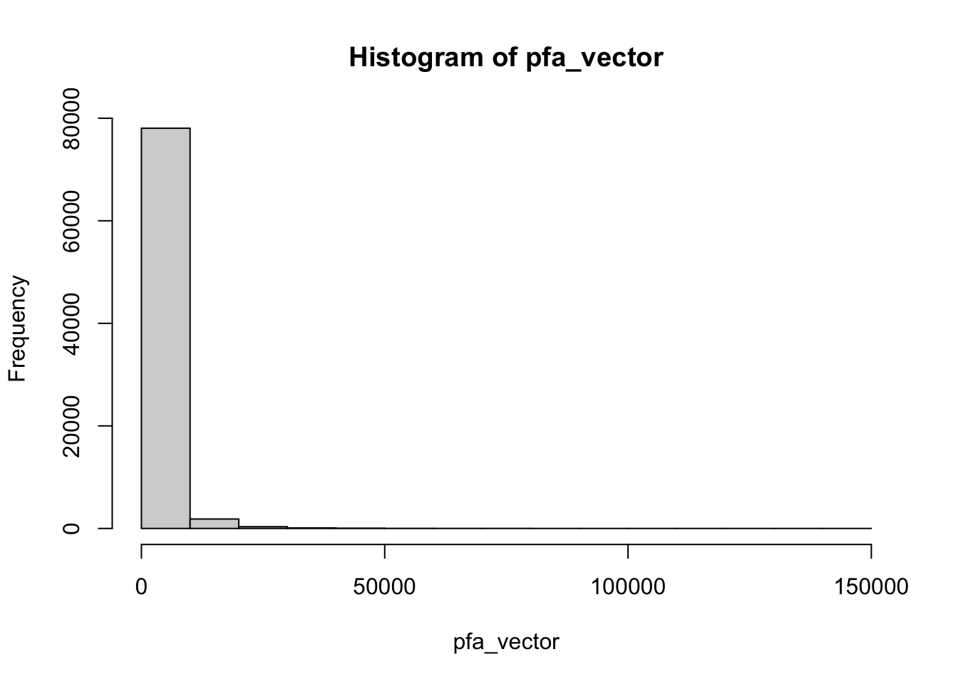

Let us now improve the histogram to get an intuition of our data. A first step is to increase the number of bins, with the

hist(pfa_vector, breaks = 200)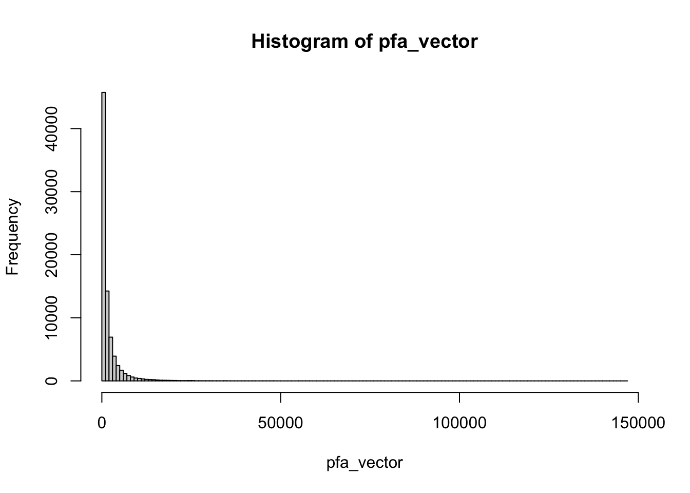

The distribution is stronly right-skewed, and its most representative part is “compressed” on the left side of the graph. As shown below, a log2 transformation provides a more informative view of the data.

## Plot the histogram of log2-transformed proteome data
## Note: we add an epsilon of 0.1 in order to avoid problems with null values
hist(log2(pfa_vector + 0.1), breaks = 100)

Enhancing the figure

## Improve the histogram
## - add a title, axis labels, coloring, ...
## - increase readaility by writing each parameter on a separate line
hist(log2(pfa_vector + 0.1), 
     breaks = seq(from = -4, to = 20, by = 0.1),
     col = "#BBDDFF",
     border = "#88AAFF",
     las = 1, # I like to read the labels
     xlab = "log2(x)", 
     ylab = "Number of observations", 
     main = "Proteome, folic-acid treated samples")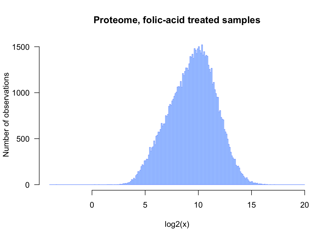

Controlling the insertion of images in an R markdown report

We will now add a some options to the header of the R chunk in the R markdown, in order to control the way this figure is inserted in the report. Note that the chunk header must come on a single line.

```{r fa_hist_log2_sized, out.width="75%", fig.width=7, fig.height=4, fig.cap="Distribution of log2-transformed values for the proteome of folic acid-treated samples (data from Pavcovic et al., 2019)"}

• fig.height and fig.width specify the size of the figure generated by R. These parameters are convenient to ensure proper proportions between height and widths, but also to incresae the readability of the labels (if you increasa the size, the fonts will look smaller).

• out.width enables you to control the width occupied by your figure in the HTML or pdf report.

• fig.cap enables you to add a caption to the figure

## Improve the histogram
## - add a title, axis labels, coloring, ...
## - increase readaility by writing each parameter on a separate line
hist(log2(pfa_vector), 
     breaks = seq(from = 0, to = 20, by = 0.1),
     col = "#BBDDFF",
     border = "#88AAFF",
     las = 1, # I like to read the labels
     xlab = "log2(x)", 
     ylab = "Number of observations", 
     main = "Proteome, folic-acid treated samples")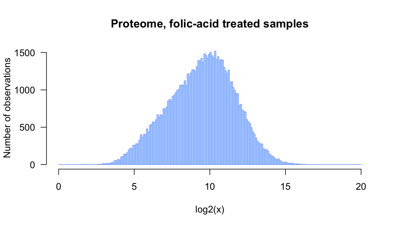

Distribution of log2-transformed values for the proteome of folic acid-treated samples (data from Pavcovic et al., 2019)

Box plots

Here is an example of code for a log2 boxplot ofthe fa data that uses the metadata tables to set up the colors.

Proteome data

## Box plot of the transcriptome data before and after normalisation
par_ori <- par(no.readonly = TRUE) ## Store the original parameters in order to restore them afterwards
par(mar = c(4, 6, 5, 1)) ## Adapt the margins of the boxplot in order to have enough space for sample labels
par(mfrow = c(1,2)) ## Two side-by-side panes

## Compute the log2 of the proteome data
## Note: we add an epsilon of 0.1 to avoid problems with null values
log2pfa <- log2(pfa + 0.1)

boxplot(pfa, 
        col = pfa_metadata$color,
        horizontal = TRUE, 
        las = 1, 
        main = "Proteome, original values", 
        xlab = "value")


boxplot(log2pfa, 
        col = pfa_metadata$color,
        horizontal = TRUE, 
        las = 1, 
        main = "Proteome, log2-transformed", 
        xlab = "log2(value)")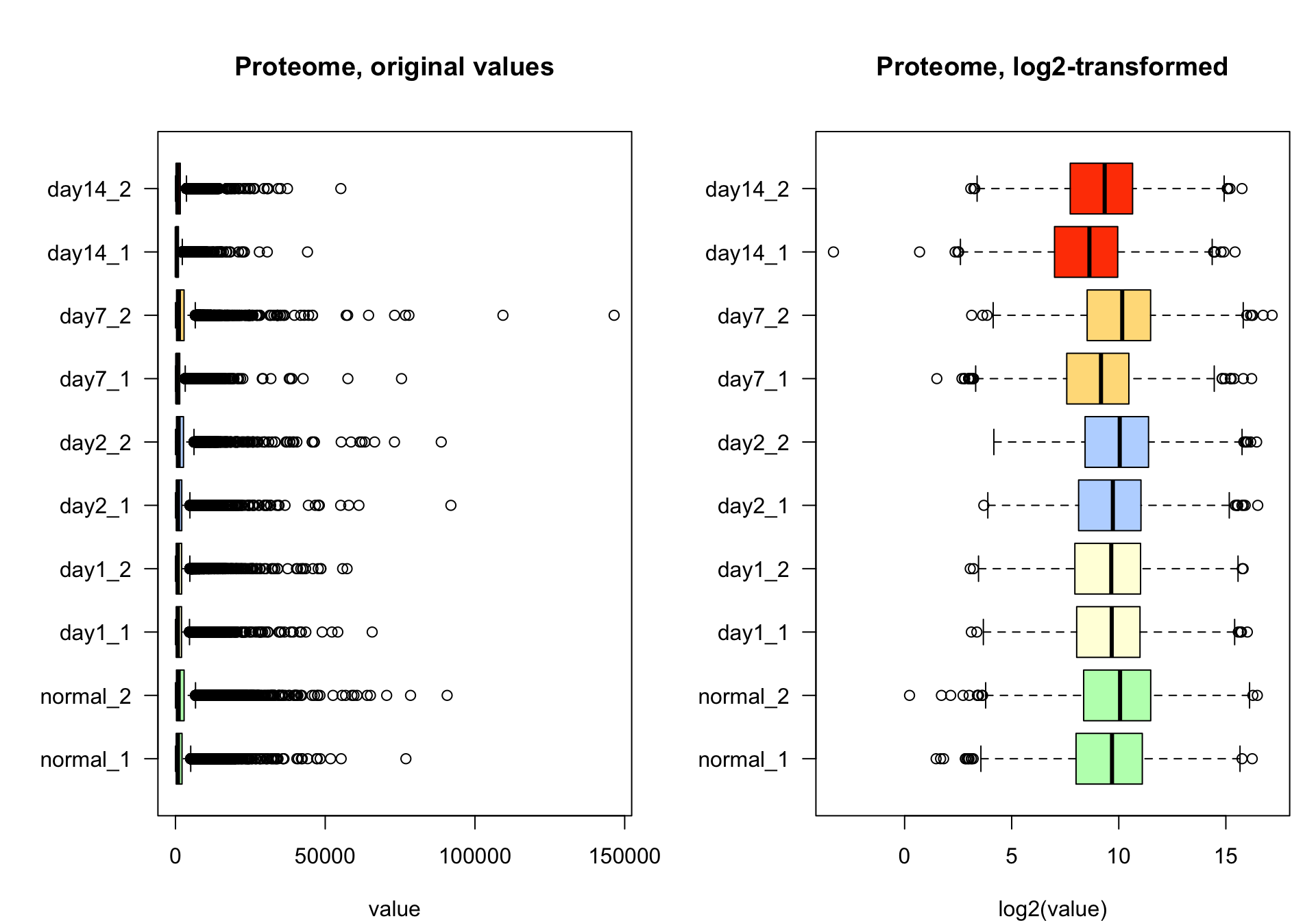

Box plots of proteome data before (left) and after (right) log2 transformation.

par(par_ori)

The box plots show the distribution of the data before (left) and after (right) log2 transformation.

Transcriptome data

The transcriptome data is providedd

## Box plot of the transcriptome data before and after normalisation
par_ori <- par(no.readonly = TRUE) ## Store the original parameters in order to restore them afterwards
par(mar = c(4, 6, 5, 1)) ## Adapt the margins of the boxplot in order to have enough space for sample labels
par(mfrow = c(2,2)) ## 4 panels, with 2 rows and 2 columns

## Counts before and after normalisation, but no log2 transformation

## Raw counts
boxplot(fa, 
        col = fa_metadata$color,
        horizontal = TRUE, 
        las = 1, 
        main = "FA transcriptome\nraw counts", 
        xlab = "counts")

## Normalised transcriptome data
boxplot(fa_norm, 
        col = fa_metadata$color,
        horizontal = TRUE, 
        las = 1, 
        main = "FA transcriptome\nnormalised counts", 
        xlab = "counts")


## Compute the log2 of the transcriptome data
## Note: we add an epsilon of 0.1 to avoid problems with null values
log2fa <- log2(fa + 0.1)
log2fa_norm <- log2(fa_norm + 0.1)

## Raw counts
boxplot(log2fa, 
        col = fa_metadata$color,
        horizontal = TRUE, 
        las = 1, 
        main = "FA transcriptome\nlog2raw (counts)", 
        xlab = "log2(counts)")

## Normalised transcriptome data
boxplot(log2fa_norm, 
        col = fa_metadata$color,
        horizontal = TRUE, 
        las = 1, 
        main = "FA transcriptome\nlog2(normalised counts)", 
        xlab = "log2(normalised counts)")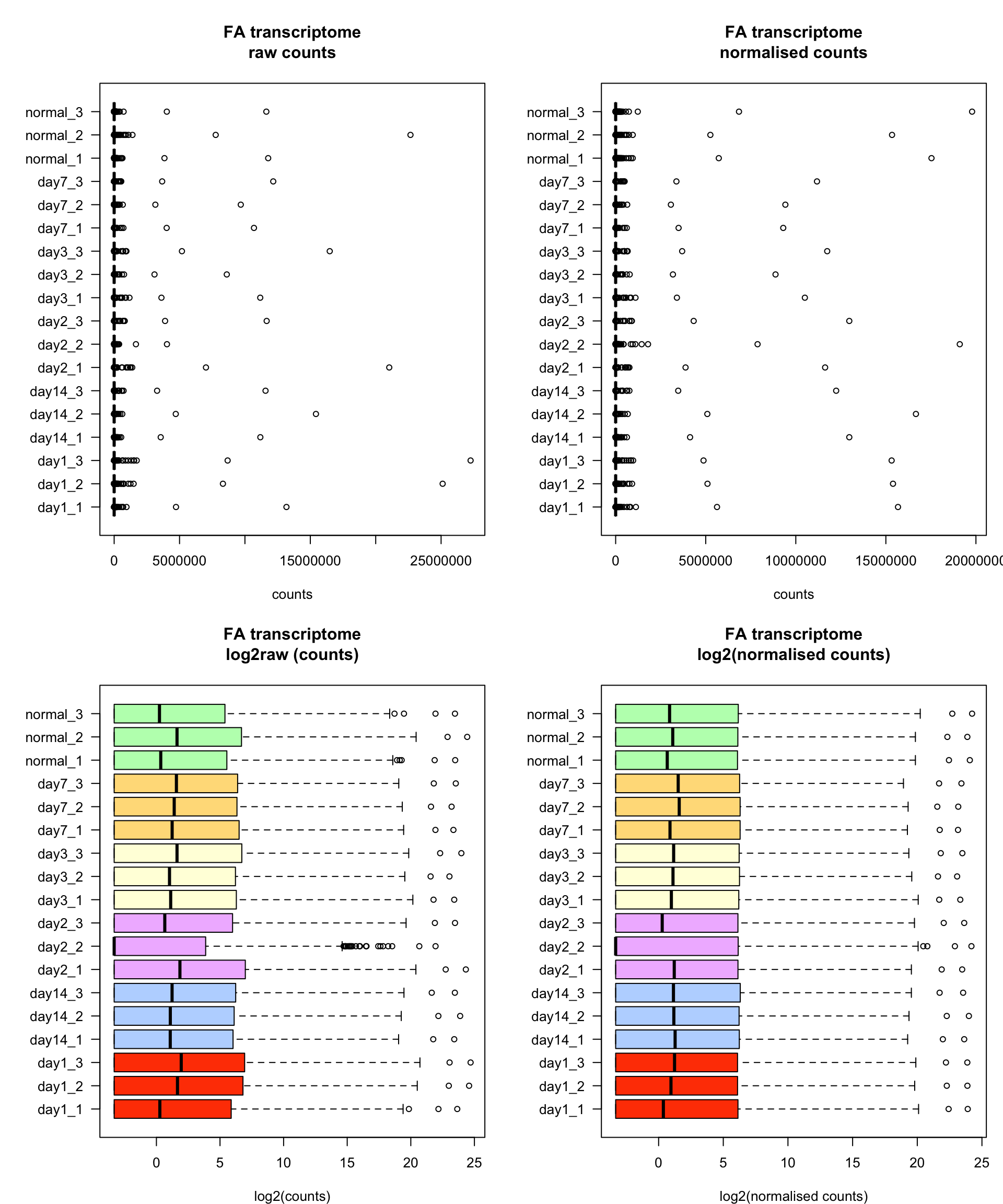

Box plots of transcriptome data before (left) and after (right) normalisation. All values are log2 transformed.

par(par_ori)

Observations

1. The raw and normalised counts (top) show a strongly right-skewed distribution due to the presence of outliers. In each sample, a very few genes have very high values (25 miilion counts !). Such outliers can be really problematic because they will exert a very strong effect on the subsequent analyses (PCA, clustering, or any other analysis that relies on distances between samples). For PCA, we recommend to use the log2-transformed values.

2. The log2 transformation (bottom) mittigates the impact of these outliers. The bottom right panel shows that all the samples have the same third quartile (right side of the boxplot rectangle), thereby indicating the method used to standardise this method.

3. For all samples, the third quartile equals the minimal value, indicating that at least 25% of the genes had a null count.

4. The sample day2_2 has a median value equal to its minimal value, indicating that at least 50% of the genes have null value in this sample.

Exercise: PCA of Pavkovicz data

As an exercise, we ask you to insert here your analysis of Pavkovicz data with the PCA methods presented in the session 4 of this course. Try to generate nice figures that will give you insight into the structure of the 4 datasets : transcriptome and proteome for the two respective treatments (folic acid and surgery, respectively).

For this, you should first download a copy of the R markdown source, install it in a local folder, and run knitr to compile an HTML or pdf report. If this works, you will start adding your own chunks of code and interpretation of the results.

Tips: - play with the scale options of the PC transformation - test if the 3rd and 4th components provide additional information than the 1st and 2nd components - compare the results obtained with the raw and normalised data sets, respectively - test the PCA with and without log2 transformation

It is not necessary to show all the results in this report, only select the most informative plots.

At the end, we expect to find here the most relevant figures resulting from this exploration, with a short explanation of - the parameters you chose for the analysis (normalised or not, log2 transformed or not, PC scaling or not, …) - some interpretation of the results in term of positioning of the samples on the components.

Don’t hesitate to call the team in case of trouble.

Save a memory image of your session

Use the function save.image() to store an image of your session, in a file pavkovic_memory_image.Rdata in the local folder specified above. This file will contain all the data that you loaded during this session, and enable you to reload everything without having to re-execute all the steps.

## Define the path to the memory image file
memory_image_file <- file.path(local_folder, "pavkovic_memory_image.Rdata")

## Save the memory image
save.image(file = memory_image_file)

message("Memory image saved in file\n\t", memory_image_file)

For a future session, you will be able to reload all the data with a single command:

load([path_to_your_memory_image])

You will need to replace [path_to_your_memory_image] by your actual path. In my case, the command becomes:

load("~/DUBii-m3_data/pavkovic_2019/pavkovic_memory_image.Rdata")

Save your session info

For the sake of traceability, store the specifications of your R environment in the report, with the command sessionInfo(). This will indicate the version of R as wella sof all the libraries used in this notebook.

sessionInfo()

R version 4.0.2 (2020-06-22)
Platform: x86_64-apple-darwin17.0 (64-bit)
Running under: macOS Mojave 10.14.6

Matrix products: default
BLAS:   /Library/Frameworks/R.framework/Versions/4.0/Resources/lib/libRblas.dylib
LAPACK: /Library/Frameworks/R.framework/Versions/4.0/Resources/lib/libRlapack.dylib

locale:
[1] en_US.UTF-8/en_US.UTF-8/en_US.UTF-8/C/en_US.UTF-8/en_US.UTF-8

attached base packages:
[1] stats     graphics  grDevices utils     datasets  methods   base     

other attached packages:
[1] knitr_1.31

loaded via a namespace (and not attached):
 [1] digest_0.6.27     R6_2.5.0          jsonlite_1.7.2    magrittr_2.0.1    evaluate_0.14     highr_0.8         rlang_0.4.10      stringi_1.5.3     jquerylib_0.1.3   bslib_0.2.4       rmarkdown_2.7     tools_4.0.2       stringr_1.4.0     xfun_0.22         yaml_2.2.1        compiler_4.0.2   
[17] htmltools_0.5.1.1 sass_0.3.1