Tutorial: machine-learning with TGCA BIC transcriptome
01. Data loading
Jacques van Helden
2021-03-29
Downloading and loading the data and metadata files
The preprocessed datasets are available on the course github repository.
A convenient function to download files only once
We will use the function download_only_once() that we defined in a previous course on data exploration.
This function takes as input a base URL, a file name and a local folder.
- It checks if the local folder already exists, and if not creates it.
- It then checks if the file is already present in this local folder, and if not downloads it.
This facilitates the downloading of the different files required for the practical. Open the code box below and run the code in your R console.
#' @title Download a file only if it is not yet here
#' @author Jacques van Helden email{Jacques.van-Helden@@france-bioinformatique.fr}
#' @param url_base base of the URL, that will be prepended to the file name
#' @param file_name name of the file (should not contain any path)
#' @param local_folder path of a local folder where the file should be stored
#' @return the function returns the path of the local file, built from local_folder and file_name
#' @export©
download_only_once <- function(
  url_base,
  file_name,
  local_folder) {

  ## Define the source URL
  url <- file.path(url_base, file_name)
  message("Source URL\n\t",  url)

  ## Define the local file
  local_file <- file.path(local_folder, file_name)

  ## Create the local data folder if it does not exist
  dir.create(local_folder, showWarnings = FALSE, recursive = TRUE)

  ## Download the file ONLY if it is not already there
  if (!file.exists(local_file)) {
    message("Downloading file from source URL to local file\n\t",
            local_file)
    download.file(url = url, destfile = local_file)
  } else {
    message("Local file already exists, no need to download\n\t",
            local_file)
  }

  return(local_file)
}
Exercise: data download
- Use the function
download_only_once()to download the BIC transciptome data and metadata from the github web site and store it in a local folder (for example~/m3-stat-R/TCGA-BIC_analysis).
Base URL: https://github.com/DU-Bii/module-3-Stat-R/raw/master/stat-R_2021/data/TCGA_BIC_subset/
Files :
Expression table (1000 top-ranking genes from differential analysis):
File name:
BIC_log2-norm-counts_edgeR_DEG_top_1000.tsv.gzThis file contains log2-transformed and standardised counts, with 1000 genes (rows) x 819 samples (columns)
Metadata:
File name:
BIC_sample-classes.tsv.gzThis file indicates the status of the 3 marker genes traditionnally used to diagnose the breast cancer type, as well as the cancer class derived from these 3 markers
For more information, see the pre-processing report: import_TCGA_from_Recount.html
- After having downloaded these files, load them in variables having the following names (for the sake of consistency with the course material).
- Expression table: bic_expr
- Metadata: bic_meta
Solution: data download and load
## Define the remote URL and local folder
bic_url <- "https://github.com/DU-Bii/module-3-Stat-R/raw/master/stat-R_2021/data/TCGA_BIC_subset/"

bic_folder <- "~/m3-stat-R/TCGA-BIC_analysis"

## Download and load the expression data table
## Note: we use check.names=FALSE to avoid replacing hyphens by dots
## in sample names, because we want to keep them as in the
## original data files.
bic_expr_file <- download_only_once(
  url_base = bic_url,
  file_name = "BIC_log2-norm-counts_edgeR_DEG_top_1000.tsv.gz",
  local_folder = bic_folder)
bic_expr <- read.delim(file = bic_expr_file,
                       header = TRUE,
                       row.names = 1,
                       check.names = FALSE)
# colnames(bic_expr)
# dim(bic_expr)
# View(head(bic_expr))

## Download the metadata file
bic_meta_file <- download_only_once(
  url_base = bic_url,
  file_name = "BIC_sample-classes.tsv.gz",
  local_folder = bic_folder)
bic_meta <- read.delim(file = bic_meta_file,
                       header = TRUE,
                       row.names = 1,
                       check.names = FALSE)
Exploring the metadata
Exercise: metadata exploration
Check the content of the metadata file by looking at the first rows, and count the number of samples per class.
Solution: metadata exploration
## Show the head of the metadata table
kable(head(bic_meta, n = 10), caption = "First rows of the BIC metadata table")| cancer.type | ER1 | PR1 | Her2 | |
|---|---|---|---|---|
| 1AB92ADA-637E-4A42-A39A-70CEEEA41AE3 | Luminal.A | Positive | Positive | Negative |
| DA98A67C-F11F-41D3-8223-1161EBFF8B58 | Unclassified | Positive | Negative | Negative |
| 06CCFD0F-7FB8-471E-B823-C7876582D6FC | HER2pos | Negative | Negative | Positive |
| A33B2F42-6EC6-4FB2-8BE5-542407A0382E | Unclassified | Positive | Negative | Negative |
| D021A258-8713-4383-9DCA-45E2F54A0411 | Luminal.A | Positive | Positive | Negative |
| C705FA90-D9AA-4949-BACA-1C022A14CB03 | Luminal.A | Positive | Positive | Negative |
| 85380A2D-9951-4D4B-A2A4-6F5F2AFC54E3 | Luminal.A | Positive | Positive | Negative |
| F53A9C63-1AF7-4CBC-B8B7-4AA7AAED3364 | Luminal.A | Positive | Positive | Negative |
| 13EF5323-EAD9-4BC7-8AC4-33875BF12E17 | Luminal.B | Positive | Positive | Positive |
| 079EACA1-0319-4B54-B20B-673F4576C69D | Basal.like | Negative | Negative | Negative |
## Number of samples per class
kable(sort(table(bic_meta$cancer.type), decreasing = TRUE),
caption = "Number of samples per class")| Var1 | Freq |
|---|---|
| Luminal.A | 422 |
| Basal.like | 131 |
| Luminal.B | 118 |
| Unclassified | 107 |
| HER2pos | 41 |
Sorting samples by cancer class
Sort the expression and metadata tables so that the samples with the same class come together. This is a bit triccky so we provide immediately the solution, but you might attempt todo it in you way if you have time.
Some tips: sorting samples
The expression table has one row per gene and one column per sample, whereas the metadata file has one row per sample.
You can use the function
order()to obtain the indices of the metadata table by order of sample class. This will return a vector with all the indixes of the first class, then all the indices of the second class, etc.You can then use the indices of the dataframes to re-order them.
We are not sure that the samples have the same order in the metadata and in the expression tables. So we will use the sample class to re-order the rows (samples) of the metadata file, but after this is done we will use the sample IDs of the metadata file (in the row names) in order to sort the columns of the expression table. This will guarantee that samples are in a consistent order between data and metadata tables.
Solution: sorting samples
## Check that the row names of the metadata contain the same set
## of IDs than the column names of the expression table
length(rownames(bic_meta)) ## the metadata contains 819 rows
[1] 819length(colnames(bic_expr)) ## the data contains 819 columns[1] 819length(intersect(rownames(bic_meta), colnames(bic_expr))) ## Their intersection contains the same number of elements[1] 819## Get the sample order according to the cancer type column of the metadata
sample_order <- order(bic_meta$cancer.type)
print(bic_meta$cancer.type[sample_order]) [1] "Basal.like" "Basal.like" "Basal.like" "Basal.like" "Basal.like" "Basal.like" "Basal.like" "Basal.like" "Basal.like" "Basal.like" "Basal.like" "Basal.like" "Basal.like" "Basal.like" "Basal.like" "Basal.like" "Basal.like" "Basal.like" "Basal.like"
[20] "Basal.like" "Basal.like" "Basal.like" "Basal.like" "Basal.like" "Basal.like" "Basal.like" "Basal.like" "Basal.like" "Basal.like" "Basal.like" "Basal.like" "Basal.like" "Basal.like" "Basal.like" "Basal.like" "Basal.like" "Basal.like" "Basal.like"
[39] "Basal.like" "Basal.like" "Basal.like" "Basal.like" "Basal.like" "Basal.like" "Basal.like" "Basal.like" "Basal.like" "Basal.like" "Basal.like" "Basal.like" "Basal.like" "Basal.like" "Basal.like" "Basal.like" "Basal.like" "Basal.like" "Basal.like"
[58] "Basal.like" "Basal.like" "Basal.like" "Basal.like" "Basal.like" "Basal.like" "Basal.like" "Basal.like" "Basal.like" "Basal.like" "Basal.like" "Basal.like" "Basal.like" "Basal.like" "Basal.like" "Basal.like" "Basal.like" "Basal.like" "Basal.like"
[77] "Basal.like" "Basal.like" "Basal.like" "Basal.like" "Basal.like" "Basal.like" "Basal.like" "Basal.like" "Basal.like" "Basal.like" "Basal.like" "Basal.like" "Basal.like" "Basal.like" "Basal.like" "Basal.like" "Basal.like" "Basal.like" "Basal.like"
[96] "Basal.like" "Basal.like" "Basal.like" "Basal.like" "Basal.like" "Basal.like" "Basal.like" "Basal.like" "Basal.like" "Basal.like" "Basal.like" "Basal.like" "Basal.like" "Basal.like" "Basal.like" "Basal.like" "Basal.like" "Basal.like" "Basal.like"
[115] "Basal.like" "Basal.like" "Basal.like" "Basal.like" "Basal.like" "Basal.like" "Basal.like" "Basal.like" "Basal.like" "Basal.like" "Basal.like" "Basal.like" "Basal.like" "Basal.like" "Basal.like" "Basal.like" "Basal.like" "HER2pos" "HER2pos"
[134] "HER2pos" "HER2pos" "HER2pos" "HER2pos" "HER2pos" "HER2pos" "HER2pos" "HER2pos" "HER2pos" "HER2pos" "HER2pos" "HER2pos" "HER2pos" "HER2pos" "HER2pos" "HER2pos" "HER2pos" "HER2pos" "HER2pos"
[153] "HER2pos" "HER2pos" "HER2pos" "HER2pos" "HER2pos" "HER2pos" "HER2pos" "HER2pos" "HER2pos" "HER2pos" "HER2pos" "HER2pos" "HER2pos" "HER2pos" "HER2pos" "HER2pos" "HER2pos" "HER2pos" "HER2pos"
[172] "HER2pos" "Luminal.A" "Luminal.A" "Luminal.A" "Luminal.A" "Luminal.A" "Luminal.A" "Luminal.A" "Luminal.A" "Luminal.A" "Luminal.A" "Luminal.A" "Luminal.A" "Luminal.A" "Luminal.A" "Luminal.A" "Luminal.A" "Luminal.A" "Luminal.A"
[191] "Luminal.A" "Luminal.A" "Luminal.A" "Luminal.A" "Luminal.A" "Luminal.A" "Luminal.A" "Luminal.A" "Luminal.A" "Luminal.A" "Luminal.A" "Luminal.A" "Luminal.A" "Luminal.A" "Luminal.A" "Luminal.A" "Luminal.A" "Luminal.A" "Luminal.A"
[210] "Luminal.A" "Luminal.A" "Luminal.A" "Luminal.A" "Luminal.A" "Luminal.A" "Luminal.A" "Luminal.A" "Luminal.A" "Luminal.A" "Luminal.A" "Luminal.A" "Luminal.A" "Luminal.A" "Luminal.A" "Luminal.A" "Luminal.A" "Luminal.A" "Luminal.A"
[229] "Luminal.A" "Luminal.A" "Luminal.A" "Luminal.A" "Luminal.A" "Luminal.A" "Luminal.A" "Luminal.A" "Luminal.A" "Luminal.A" "Luminal.A" "Luminal.A" "Luminal.A" "Luminal.A" "Luminal.A" "Luminal.A" "Luminal.A" "Luminal.A" "Luminal.A"
[248] "Luminal.A" "Luminal.A" "Luminal.A" "Luminal.A" "Luminal.A" "Luminal.A" "Luminal.A" "Luminal.A" "Luminal.A" "Luminal.A" "Luminal.A" "Luminal.A" "Luminal.A" "Luminal.A" "Luminal.A" "Luminal.A" "Luminal.A" "Luminal.A" "Luminal.A"
[267] "Luminal.A" "Luminal.A" "Luminal.A" "Luminal.A" "Luminal.A" "Luminal.A" "Luminal.A" "Luminal.A" "Luminal.A" "Luminal.A" "Luminal.A" "Luminal.A" "Luminal.A" "Luminal.A" "Luminal.A" "Luminal.A" "Luminal.A" "Luminal.A" "Luminal.A"
[286] "Luminal.A" "Luminal.A" "Luminal.A" "Luminal.A" "Luminal.A" "Luminal.A" "Luminal.A" "Luminal.A" "Luminal.A" "Luminal.A" "Luminal.A" "Luminal.A" "Luminal.A" "Luminal.A" "Luminal.A" "Luminal.A" "Luminal.A" "Luminal.A" "Luminal.A"
[305] "Luminal.A" "Luminal.A" "Luminal.A" "Luminal.A" "Luminal.A" "Luminal.A" "Luminal.A" "Luminal.A" "Luminal.A" "Luminal.A" "Luminal.A" "Luminal.A" "Luminal.A" "Luminal.A" "Luminal.A" "Luminal.A" "Luminal.A" "Luminal.A" "Luminal.A"
[324] "Luminal.A" "Luminal.A" "Luminal.A" "Luminal.A" "Luminal.A" "Luminal.A" "Luminal.A" "Luminal.A" "Luminal.A" "Luminal.A" "Luminal.A" "Luminal.A" "Luminal.A" "Luminal.A" "Luminal.A" "Luminal.A" "Luminal.A" "Luminal.A" "Luminal.A"
[343] "Luminal.A" "Luminal.A" "Luminal.A" "Luminal.A" "Luminal.A" "Luminal.A" "Luminal.A" "Luminal.A" "Luminal.A" "Luminal.A" "Luminal.A" "Luminal.A" "Luminal.A" "Luminal.A" "Luminal.A" "Luminal.A" "Luminal.A" "Luminal.A" "Luminal.A"
[362] "Luminal.A" "Luminal.A" "Luminal.A" "Luminal.A" "Luminal.A" "Luminal.A" "Luminal.A" "Luminal.A" "Luminal.A" "Luminal.A" "Luminal.A" "Luminal.A" "Luminal.A" "Luminal.A" "Luminal.A" "Luminal.A" "Luminal.A" "Luminal.A" "Luminal.A"
[381] "Luminal.A" "Luminal.A" "Luminal.A" "Luminal.A" "Luminal.A" "Luminal.A" "Luminal.A" "Luminal.A" "Luminal.A" "Luminal.A" "Luminal.A" "Luminal.A" "Luminal.A" "Luminal.A" "Luminal.A" "Luminal.A" "Luminal.A" "Luminal.A" "Luminal.A"
[400] "Luminal.A" "Luminal.A" "Luminal.A" "Luminal.A" "Luminal.A" "Luminal.A" "Luminal.A" "Luminal.A" "Luminal.A" "Luminal.A" "Luminal.A" "Luminal.A" "Luminal.A" "Luminal.A" "Luminal.A" "Luminal.A" "Luminal.A" "Luminal.A" "Luminal.A"
[419] "Luminal.A" "Luminal.A" "Luminal.A" "Luminal.A" "Luminal.A" "Luminal.A" "Luminal.A" "Luminal.A" "Luminal.A" "Luminal.A" "Luminal.A" "Luminal.A" "Luminal.A" "Luminal.A" "Luminal.A" "Luminal.A" "Luminal.A" "Luminal.A" "Luminal.A"
[438] "Luminal.A" "Luminal.A" "Luminal.A" "Luminal.A" "Luminal.A" "Luminal.A" "Luminal.A" "Luminal.A" "Luminal.A" "Luminal.A" "Luminal.A" "Luminal.A" "Luminal.A" "Luminal.A" "Luminal.A" "Luminal.A" "Luminal.A" "Luminal.A" "Luminal.A"
[457] "Luminal.A" "Luminal.A" "Luminal.A" "Luminal.A" "Luminal.A" "Luminal.A" "Luminal.A" "Luminal.A" "Luminal.A" "Luminal.A" "Luminal.A" "Luminal.A" "Luminal.A" "Luminal.A" "Luminal.A" "Luminal.A" "Luminal.A" "Luminal.A" "Luminal.A"
[476] "Luminal.A" "Luminal.A" "Luminal.A" "Luminal.A" "Luminal.A" "Luminal.A" "Luminal.A" "Luminal.A" "Luminal.A" "Luminal.A" "Luminal.A" "Luminal.A" "Luminal.A" "Luminal.A" "Luminal.A" "Luminal.A" "Luminal.A" "Luminal.A" "Luminal.A"
[495] "Luminal.A" "Luminal.A" "Luminal.A" "Luminal.A" "Luminal.A" "Luminal.A" "Luminal.A" "Luminal.A" "Luminal.A" "Luminal.A" "Luminal.A" "Luminal.A" "Luminal.A" "Luminal.A" "Luminal.A" "Luminal.A" "Luminal.A" "Luminal.A" "Luminal.A"
[514] "Luminal.A" "Luminal.A" "Luminal.A" "Luminal.A" "Luminal.A" "Luminal.A" "Luminal.A" "Luminal.A" "Luminal.A" "Luminal.A" "Luminal.A" "Luminal.A" "Luminal.A" "Luminal.A" "Luminal.A" "Luminal.A" "Luminal.A" "Luminal.A" "Luminal.A"
[533] "Luminal.A" "Luminal.A" "Luminal.A" "Luminal.A" "Luminal.A" "Luminal.A" "Luminal.A" "Luminal.A" "Luminal.A" "Luminal.A" "Luminal.A" "Luminal.A" "Luminal.A" "Luminal.A" "Luminal.A" "Luminal.A" "Luminal.A" "Luminal.A" "Luminal.A"
[552] "Luminal.A" "Luminal.A" "Luminal.A" "Luminal.A" "Luminal.A" "Luminal.A" "Luminal.A" "Luminal.A" "Luminal.A" "Luminal.A" "Luminal.A" "Luminal.A" "Luminal.A" "Luminal.A" "Luminal.A" "Luminal.A" "Luminal.A" "Luminal.A" "Luminal.A"
[571] "Luminal.A" "Luminal.A" "Luminal.A" "Luminal.A" "Luminal.A" "Luminal.A" "Luminal.A" "Luminal.A" "Luminal.A" "Luminal.A" "Luminal.A" "Luminal.A" "Luminal.A" "Luminal.A" "Luminal.A" "Luminal.A" "Luminal.A" "Luminal.A" "Luminal.A"
[590] "Luminal.A" "Luminal.A" "Luminal.A" "Luminal.A" "Luminal.A" "Luminal.B" "Luminal.B" "Luminal.B" "Luminal.B" "Luminal.B" "Luminal.B" "Luminal.B" "Luminal.B" "Luminal.B" "Luminal.B" "Luminal.B" "Luminal.B" "Luminal.B" "Luminal.B"
[609] "Luminal.B" "Luminal.B" "Luminal.B" "Luminal.B" "Luminal.B" "Luminal.B" "Luminal.B" "Luminal.B" "Luminal.B" "Luminal.B" "Luminal.B" "Luminal.B" "Luminal.B" "Luminal.B" "Luminal.B" "Luminal.B" "Luminal.B" "Luminal.B" "Luminal.B"
[628] "Luminal.B" "Luminal.B" "Luminal.B" "Luminal.B" "Luminal.B" "Luminal.B" "Luminal.B" "Luminal.B" "Luminal.B" "Luminal.B" "Luminal.B" "Luminal.B" "Luminal.B" "Luminal.B" "Luminal.B" "Luminal.B" "Luminal.B" "Luminal.B" "Luminal.B"
[647] "Luminal.B" "Luminal.B" "Luminal.B" "Luminal.B" "Luminal.B" "Luminal.B" "Luminal.B" "Luminal.B" "Luminal.B" "Luminal.B" "Luminal.B" "Luminal.B" "Luminal.B" "Luminal.B" "Luminal.B" "Luminal.B" "Luminal.B" "Luminal.B" "Luminal.B"
[666] "Luminal.B" "Luminal.B" "Luminal.B" "Luminal.B" "Luminal.B" "Luminal.B" "Luminal.B" "Luminal.B" "Luminal.B" "Luminal.B" "Luminal.B" "Luminal.B" "Luminal.B" "Luminal.B" "Luminal.B" "Luminal.B" "Luminal.B" "Luminal.B" "Luminal.B"
[685] "Luminal.B" "Luminal.B" "Luminal.B" "Luminal.B" "Luminal.B" "Luminal.B" "Luminal.B" "Luminal.B" "Luminal.B" "Luminal.B" "Luminal.B" "Luminal.B" "Luminal.B" "Luminal.B" "Luminal.B" "Luminal.B" "Luminal.B" "Luminal.B" "Luminal.B"
[704] "Luminal.B" "Luminal.B" "Luminal.B" "Luminal.B" "Luminal.B" "Luminal.B" "Luminal.B" "Luminal.B" "Luminal.B" "Unclassified" "Unclassified" "Unclassified" "Unclassified" "Unclassified" "Unclassified" "Unclassified" "Unclassified" "Unclassified" "Unclassified"
[723] "Unclassified" "Unclassified" "Unclassified" "Unclassified" "Unclassified" "Unclassified" "Unclassified" "Unclassified" "Unclassified" "Unclassified" "Unclassified" "Unclassified" "Unclassified" "Unclassified" "Unclassified" "Unclassified" "Unclassified" "Unclassified" "Unclassified"
[742] "Unclassified" "Unclassified" "Unclassified" "Unclassified" "Unclassified" "Unclassified" "Unclassified" "Unclassified" "Unclassified" "Unclassified" "Unclassified" "Unclassified" "Unclassified" "Unclassified" "Unclassified" "Unclassified" "Unclassified" "Unclassified" "Unclassified"
[761] "Unclassified" "Unclassified" "Unclassified" "Unclassified" "Unclassified" "Unclassified" "Unclassified" "Unclassified" "Unclassified" "Unclassified" "Unclassified" "Unclassified" "Unclassified" "Unclassified" "Unclassified" "Unclassified" "Unclassified" "Unclassified" "Unclassified"
[780] "Unclassified" "Unclassified" "Unclassified" "Unclassified" "Unclassified" "Unclassified" "Unclassified" "Unclassified" "Unclassified" "Unclassified" "Unclassified" "Unclassified" "Unclassified" "Unclassified" "Unclassified" "Unclassified" "Unclassified" "Unclassified" "Unclassified"
[799] "Unclassified" "Unclassified" "Unclassified" "Unclassified" "Unclassified" "Unclassified" "Unclassified" "Unclassified" "Unclassified" "Unclassified" "Unclassified" "Unclassified" "Unclassified" "Unclassified" "Unclassified" "Unclassified" "Unclassified" "Unclassified" "Unclassified"
[818] "Unclassified" "Unclassified"## Sort the metadata rows (samples) according to this order
bic_meta <- bic_meta[sample_order, ]
## Sort the expression table to make sure that the samples (columns)
## come in the same order as the rows of the metadata table
bic_expr <- bic_expr[, row.names(bic_meta)]Generate readable sample labels
The TCGA samples have very long and structured IDs, whcih make them inconvenient to display on the type of graphs we would like to generate (box plots, PC plots, heatmaps, …).
We will thus generate readable labels, and add them as a separate column to the metadata table.
For this, we will use the class name and use the funciotn make.names() to avoid having duplicate labels (this will add a number besides the class name).
#### Sample labels ####
bic_meta$label <- make.names(
  names = bic_meta$cancer.type,
  unique = TRUE)
Get gene IDs and names
The row names of the expression table indicate the Ensembl gene ID and the version of the genome annotation (a number after the dot). This ID is quite long, and we would prefer to have more readable labels for the genes. For this, we will get the gene name (also called “gene symbol”).
#### Get gene names ####

gene_info <- data.frame(
  ENSG = sub(x = row.names(bic_expr),
             perl = TRUE,
             replacement = "",
             pattern = '\\..*'),
  row.names = row.names(bic_expr)
)
# head(gene_info)


## Get gene names from ENSEMBL using biomaRt package
library("biomaRt")
ensembl <- useMart("ensembl", dataset = "hsapiens_gene_ensembl")
ensembl_info <- getBM(attributes = c('ensembl_gene_id',
                                     'external_gene_name',
                                     'description'),
                      filters = 'ensembl_gene_id',
                      values = gene_info$ENSG,
                      mart = ensembl)
row.names(ensembl_info) <- ensembl_info$ensembl_gene_id

## Add gene name in a new column of the gene_info table
gene_info$name <- ensembl_info[gene_info$ENSG, "external_gene_name"]
gene_info$description <- ensembl_info[gene_info$ENSG, "description"]

## There is one gene with no name
# sum(is.na(gene_info$name))
## Replace undefined gene names by the gene ID
gene_info[is.na(gene_info$name), "name"] <-
  gene_info[is.na(gene_info$name), "ENSG"]

## Print the first rows of the gene info table
kable(head(gene_info, n = 10), caption = "First rows of the gene information table collected from BioMart")| ENSG | name | description | |
|---|---|---|---|
| ENSG00000000003.14 | ENSG00000000003 | TSPAN6 | tetraspanin 6 [Source:HGNC Symbol;Acc:HGNC:11858] |
| ENSG00000000419.12 | ENSG00000000419 | DPM1 | dolichyl-phosphate mannosyltransferase subunit 1, catalytic [Source:HGNC Symbol;Acc:HGNC:3005] |
| ENSG00000000457.13 | ENSG00000000457 | SCYL3 | SCY1 like pseudokinase 3 [Source:HGNC Symbol;Acc:HGNC:19285] |
| ENSG00000000460.16 | ENSG00000000460 | C1orf112 | chromosome 1 open reading frame 112 [Source:HGNC Symbol;Acc:HGNC:25565] |
| ENSG00000000938.12 | ENSG00000000938 | FGR | FGR proto-oncogene, Src family tyrosine kinase [Source:HGNC Symbol;Acc:HGNC:3697] |
| ENSG00000000971.15 | ENSG00000000971 | CFH | complement factor H [Source:HGNC Symbol;Acc:HGNC:4883] |
| ENSG00000001036.13 | ENSG00000001036 | FUCA2 | alpha-L-fucosidase 2 [Source:HGNC Symbol;Acc:HGNC:4008] |
| ENSG00000001084.10 | ENSG00000001084 | GCLC | glutamate-cysteine ligase catalytic subunit [Source:HGNC Symbol;Acc:HGNC:4311] |
| ENSG00000001167.14 | ENSG00000001167 | NFYA | nuclear transcription factor Y subunit alpha [Source:HGNC Symbol;Acc:HGNC:7804] |
| ENSG00000001460.17 | ENSG00000001460 | STPG1 | sperm tail PG-rich repeat containing 1 [Source:HGNC Symbol;Acc:HGNC:28070] |
## Export the gene info table in a TSV file
gene_info_file_tsv <- file.path(bic_folder, "BIC_top1000_gene_info.tsv")
message("Saving gene info table in TSV file\n\t",
        gene_info_file_tsv)
write.table(x = gene_info,
            file = gene_info_file_tsv,
            quote = FALSE,
            sep = "\t",
            row.names = TRUE,
            col.names = NA)

## Export the gene info table in Excel (xlsx) file
gene_info_file_xlsx <- file.path(bic_folder, "BIC_top1000_gene_info.xlsx")
message("Saving gene info table in xlsx file\n\t",
        gene_info_file_xlsx)
openxlsx::write.xlsx(x = gene_info, file = gene_info_file_xlsx)
Assign sample colors
We add here a code to assign a color to each sample according to its class.
#### Class and sample colors ####
class_names <- unique(bic_meta$cancer.type)

## Assign one color to each class
class_color <- c(
  "Basal.like" = "#DDEEFF",
  "HER2pos" = "#88FF88",
  "Luminal.A" = "#FFBB55",
  "Luminal.B" = "#EE88FF",
  "Unclassified"  = "#8888FF"
)

## Assign a color to each sample according to its class
bic_meta$color <- class_color[bic_meta$cancer.type]
# table(bic_meta$color)
Sample standardisation
We will standardise the samples using robust estimators, to avoid the impact of extreme values.
#### Sample standardisation ####

## Compute descriptive stats on the samples
bic_meta$mean <- apply(bic_expr, 2, mean)
bic_meta$sd <- apply(bic_expr, 2, sd)
bic_meta$median <- apply(bic_expr, 2, median)
bic_meta$iqr <- apply(bic_expr, 2, IQR)

## Centering on the mean
expr_median <- median(unlist(bic_expr))
bic_expr_centered <- t(t(bic_expr) - bic_meta$median) + expr_median
# dim(bic_expr)
# dim(bic_expr_centered)
# apply(bic_expr_centered, 2, median)

## Compute the IQR of the whole expression table
expr_iqr <- IQR(unlist(bic_expr_centered))

## Scale each sample based  on its IQR
bic_expr_std <- t((t(bic_expr) - unlist(bic_meta$median))
                  /  unlist(bic_meta$iqr)) * expr_iqr + expr_median
# apply(bic_expr_std, 2, IQR)
# range( apply(bic_expr_std, 2, IQR))
# range( apply(bic_expr_std, 2, median))
Dataset with readable row and column names
Create a dataset with
- gene names as row.names
- sample labels as column.names
#### Data set with readable
bic_expr_labels <- bic_expr_std
dim(bic_expr_labels)
[1] 1000 819colnames(bic_expr_labels) <- bic_meta$label
rownames(bic_expr_labels) <- make.names(gene_info$name) Box plot
Exercise: box plot
Select 30 samples at random, and draw a boxplot.
Sort the samples according to their index in the columns of the expression table (this will ensure that samples of the same class come together).
Solution: box plot
#### Box plot ####
sample_size <- 30

## select sample indices
selected_samples <- sort(sample(
  x = 1:ncol(bic_expr),
  size = sample_size,
  replace = FALSE))

## Box plots
par.ori <- par(no.readonly = TRUE)
par(mfrow = c(1, 3))
par(mar = c(5, 6, 4, 1))
## Original data
boxplot(x = bic_expr[, selected_samples],
        names = bic_meta$label[selected_samples],
        col = bic_meta$color[selected_samples],
        xlab = "log2(counts)",
        main = "Before normalisation",
        horizontal = TRUE,
        las = 1, notch = TRUE,
        cex.axis = 1)
boxplot(x = bic_expr_centered[, selected_samples],
        names = bic_meta$label[selected_samples],
        col = bic_meta$color[selected_samples],
        xlab = "log2(counts)",
        main = "Median-based centering",
        horizontal = TRUE,
        las = 1, notch = TRUE,
        cex.axis = 0.7)
boxplot(x = bic_expr_std[, selected_samples],
        names = bic_meta$label[selected_samples],
        col = bic_meta$color[selected_samples],
        xlab = "log2(counts)",
        main = "IQR-based scaling",
        horizontal = TRUE,
        las = 1, notch = TRUE,
        cex.axis = 0.7)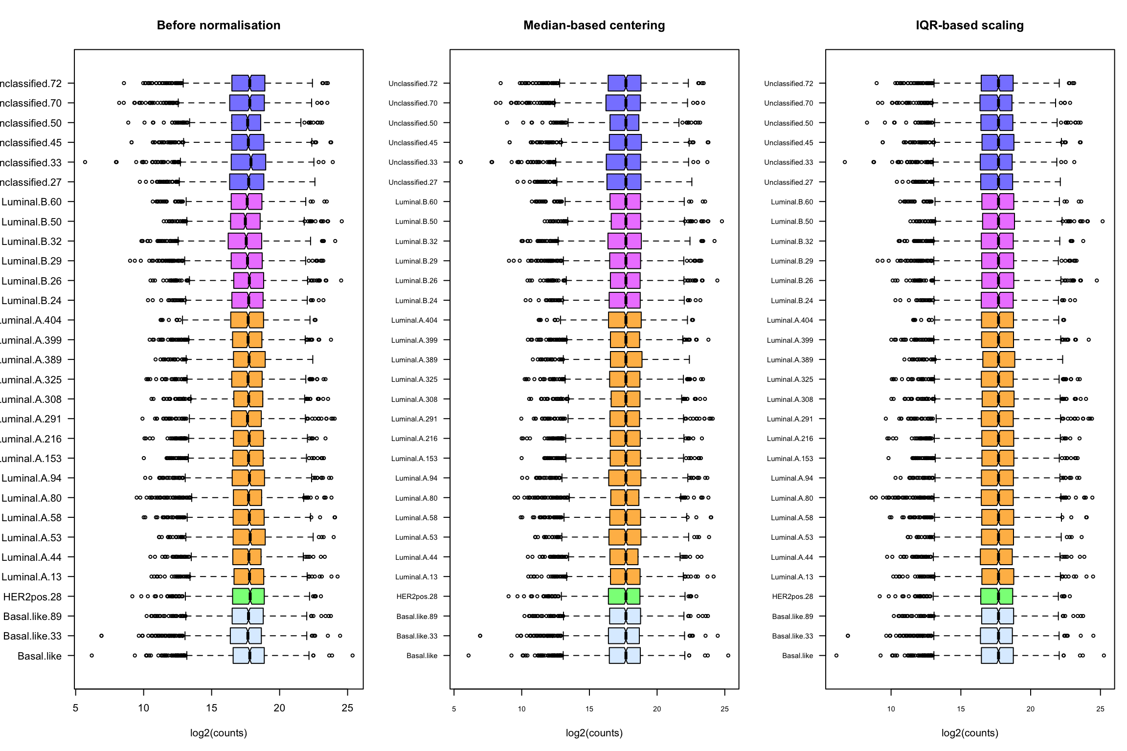
Box plot of a random selection of samples from the TCGA-BIC transcriptome dataset.
par(par.ori)PCA
Exercise
Generate a graph with the two first components and color samples according to their class. Do the sample classes segregate on this PC plot?
Solution
#### PC plot of the TAGC BIC samples ####
library(factoextra)


## Compute the principal components
## This is done on the transposed data table
bic_pca <- PCA(t(bic_expr_labels),
               scale.unit = FALSE,
               ncp = ncol(bic_expr_labels),
               graph = FALSE)

## Table with the coordinates of each sample in the PC space
bic_pcs <- bic_pca$ind$coord

# Check the PC dimensions
dim(bic_pcs)
[1] 819 818#### Plot the variance per component ####
fviz_eig(bic_pca, addlabels = TRUE)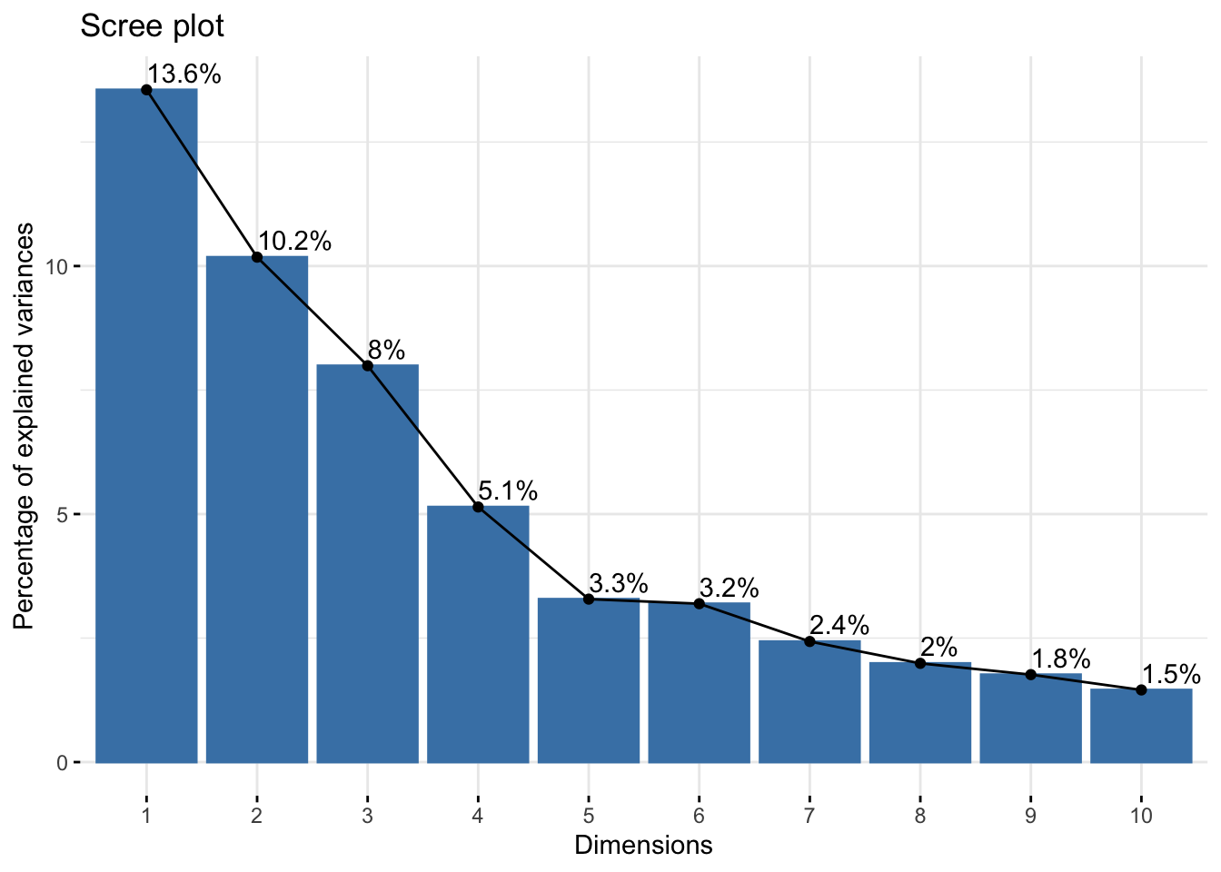
Variance of the first components for the BIC dataset
The plots of individuals show that the cancer types segregate partly onb the first and second PCs.
#### Plot individuals on the 2 first components ####
fviz_pca_ind(X = bic_pca,
             axes = c(1, 2),
             col.ind = bic_meta$cancer.type,
label = "none") 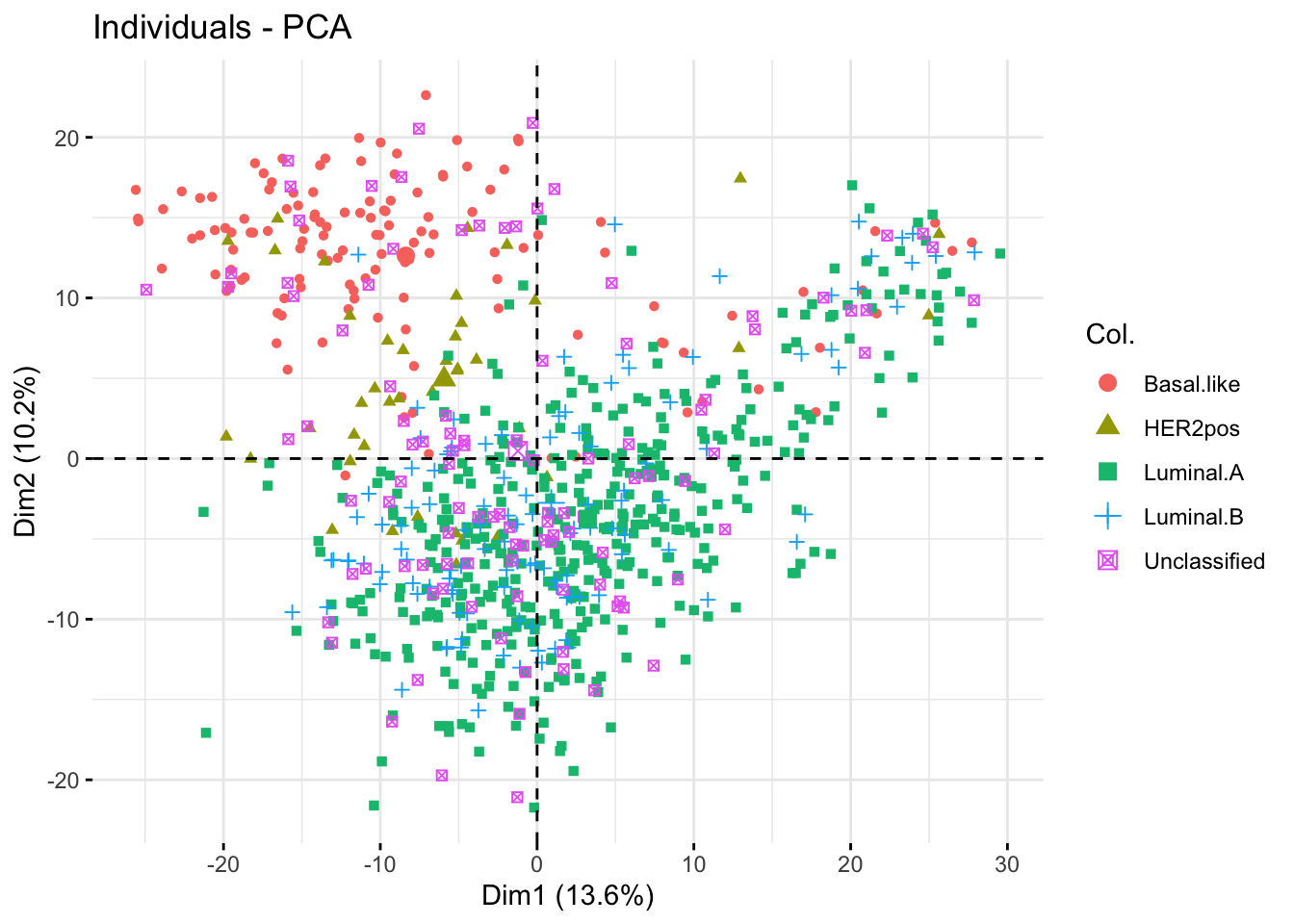
The 3rd and 4th PCs seem much less informative with respect to the cancer types: the individuals seem intermingled irrespective of their cancer type.
#### Plot individuals on the 2 first components ####
fviz_pca_ind(X = bic_pca,
             axes = c(3, 4),
             col.ind = bic_meta$cancer.type,
label = "none") 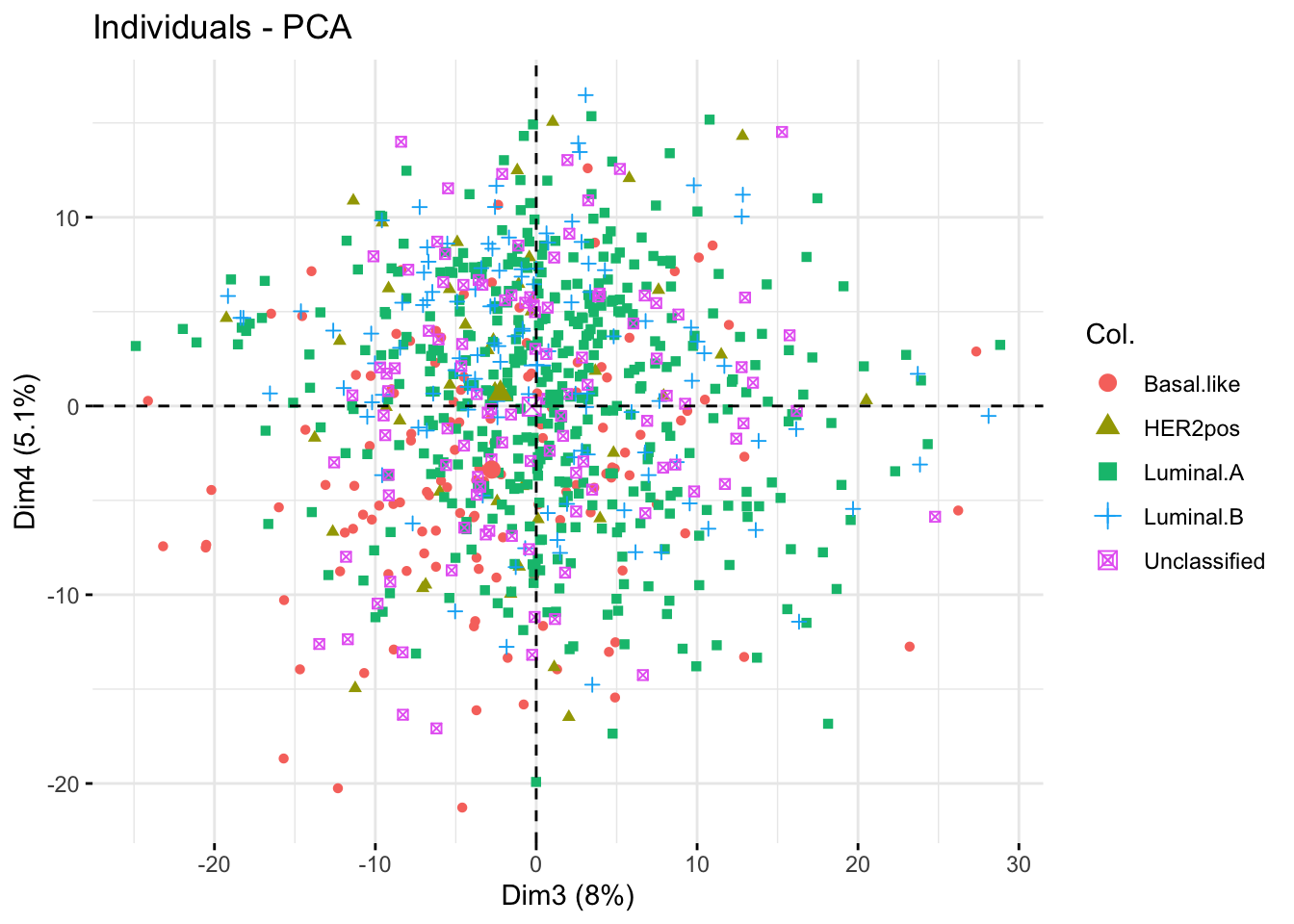
Variables
At the end of this tutorial, we dispose of the following data types.
| Variable name | Data content |
|---|---|
bic_meta |
metadata with a few added columns (sample color, estimators of central tendency and dispersion) |
gene_info |
ID, name and description of the 1000 genes used here |
bic_expr |
non-normalised expression table |
bic_expr_centered |
median-based expression table |
bic_expr_std |
sample-wise standardised expression table, all samples having the same median and IQR |
bic_expr_labels |
same content as bic_expr_std but with row names replaced by human-readable gene names, and column names by human-readable sample labels |
Save a memory image
We can now save a memory image, which will enable us to reload the whole data with a single command for the next tutorials.
#### Save memory image ####
mem_image <- file.path(bic_folder, "bic_data.Rdata")
message("Saving memory image in file\n\t", mem_image)
save.image(file = mem_image)
The memory image has been saved in a local folder, in the following file: ~/m3-stat-R/TCGA-BIC_analysis/bic_data.Rdata
Command to reload this dataset
The memory image generated at the end of this tutorial is stored on the github repository, and can be reloaded as follows.
#### Reload memory image from github repository ####
github_mem_img <- "https://github.com/DU-Bii/module-3-Stat-R/blob/master/stat-R_2021/data/TCGA_BIC_subset/bic_data.Rdata?raw=true"

## Define local destination folder
bic_folder <- "~/m3-stat-R/TCGA-BIC_analysis"
## Create it if required
dir.create(bic_folder, showWarnings = FALSE, recursive = TRUE)

## Define local destination for the memory image
mem_image <- file.path(bic_folder, "bic_data.Rdata")
if (file.exists(mem_image)) {
  message("Memory image already there, skipping download")
} else {
  message("Downloading memory image from\n", github_mem_img)
  download.file(url = github_mem_img, destfile = mem_image)
  message("Local memory image\t", mem_image)
}

## Load the memory image
message("Loading memory image", mem_image)
load(mem_image)
Session info
As usual, we write the session info in the report for the sake of traceability.
sessionInfo()R version 4.0.2 (2020-06-22)
Platform: x86_64-apple-darwin17.0 (64-bit)
Running under: macOS Mojave 10.14.6
Matrix products: default
BLAS: /Library/Frameworks/R.framework/Versions/4.0/Resources/lib/libRblas.dylib
LAPACK: /Library/Frameworks/R.framework/Versions/4.0/Resources/lib/libRlapack.dylib
locale:
[1] en_US.UTF-8/en_US.UTF-8/en_US.UTF-8/C/en_US.UTF-8/en_US.UTF-8
attached base packages:
[1] stats graphics grDevices utils datasets methods base
other attached packages:
[1] biomaRt_2.44.4 openxlsx_4.2.3 factoextra_1.0.7 ggplot2_3.3.3 FactoMineR_2.4 knitr_1.31
loaded via a namespace (and not attached):
[1] bit64_4.0.5 progress_1.2.2 httr_1.4.2 tools_4.0.2 backports_1.2.1 bslib_0.2.4 utf8_1.2.1 R6_2.5.0 DT_0.17 DBI_1.1.1 BiocGenerics_0.34.0 colorspace_2.0-0 withr_2.4.1 tidyselect_1.1.0
[15] prettyunits_1.1.1 bit_4.0.4 curl_4.3 compiler_4.0.2 Biobase_2.48.0 flashClust_1.01-2 xml2_1.3.2 labeling_0.4.2 sass_0.3.1 scales_1.1.1 askpass_1.1 rappdirs_0.3.3 stringr_1.4.0 digest_0.6.27
[29] foreign_0.8-81 rmarkdown_2.7 rio_0.5.26 pkgconfig_2.0.3 htmltools_0.5.1.1 dbplyr_2.1.0 fastmap_1.1.0 highr_0.8 htmlwidgets_1.5.3 rlang_0.4.10 readxl_1.3.1 RSQLite_2.2.5 farver_2.1.0 jquerylib_0.1.3
[43] generics_0.1.0 jsonlite_1.7.2 dplyr_1.0.5 zip_2.1.1 car_3.0-10 magrittr_2.0.1 leaps_3.1 Rcpp_1.0.6 munsell_0.5.0 S4Vectors_0.26.1 fansi_0.4.2 abind_1.4-5 lifecycle_1.0.0 scatterplot3d_0.3-41
[57] stringi_1.5.3 yaml_2.2.1 carData_3.0-4 MASS_7.3-53.1 BiocFileCache_1.12.1 grid_4.0.2 blob_1.2.1 parallel_4.0.2 ggrepel_0.9.1 forcats_0.5.1 crayon_1.4.1 lattice_0.20-41 haven_2.3.1 hms_1.0.0
[71] pillar_1.5.1 ggpubr_0.4.0 ggsignif_0.6.1 stats4_4.0.2 XML_3.99-0.6 glue_1.4.2 evaluate_0.14 data.table_1.14.0 BiocManager_1.30.12 vctrs_0.3.6 cellranger_1.1.0 gtable_0.3.0 openssl_1.4.3 purrr_0.3.4
[85] tidyr_1.1.3 assertthat_0.2.1 cachem_1.0.4 xfun_0.22 broom_0.7.5 rstatix_0.7.0 tibble_3.1.0 AnnotationDbi_1.50.3 memoise_2.0.0 IRanges_2.22.2 cluster_2.1.1 ellipsis_0.3.1