Tutorial: machine-learning with TGCA BIC transcriptome
02. Clustering
Anne Badel & Jacques van Helden
2021-04-13
Data loading
We provide hereafter a code to load the prepared data from a memory image on the github repository. This image has been generated at the end of the tutorial on data loading and exploration.
#### Reload memory image from github repository ####
github_mem_img <- "https://github.com/DU-Bii/module-3-Stat-R/blob/master/stat-R_2021/data/TCGA_BIC_subset/bic_data.Rdata?raw=true"

## Define local destination folder
bic_folder <- "~/m3-stat-R/TCGA-BIC_analysis"
## Create it if required
dir.create(bic_folder, showWarnings = FALSE, recursive = TRUE)

## Define local destination for the memory image
mem_image <- file.path(bic_folder, "bic_data.Rdata")
if (file.exists(mem_image)) {
  message("Memory image already there, skipping download")
} else {
  message("Downloading memory image from\n", github_mem_img)
  download.file(url = github_mem_img, destfile = mem_image)
  message("Local memory image\t", mem_image)
}

## Load the memory image
message("Loading memory image", mem_image)
load(mem_image)
The table below indicates the main variables loaded with this memory image.
| Variable name | Data content |
|---|---|
class_color |
a vector specifying the color to be associated to each sample class (cancer type) |
bic_meta |
metadata with a few added columns (sample color, estimators of central tendency and dispersion) |
gene_info |
ID, name and description of the 1000 genes used here |
bic_expr |
non-normalised expression table |
bic_expr_centered |
median-based expression table |
bic_expr_std |
sample-wise standardised expression table, all samples having the same median and IQR |
bic_expr_labels |
same content as bic_expr_std but with row names replaced by human-readable gene names, and column names by human-readable sample labels |
Use the command View() or head() or any other convenient way of your choice to check the content of these variables.
Subset selection
The original data table contains 819 samples (columns) x 1000 genes (rows). These dimensions are not convenient for visualisation, so we will start by selecting a smaller set of samples and genes.
Note that this smaller data subset will serve only for didactic purposes; at the end of the practical, we will apply the clustering to all the genes with all the samples, in order to get relevant results.
Exercise: subset selection
- In the metadata table, count the number of samples per cancer type.
#### Samples per cancer type ####
kable(sort(table(bic_meta$cancer.type), decreasing = TRUE),
caption = "Number of samples per cancer type")| Var1 | Freq |
|---|---|
| Luminal.A | 422 |
| Basal.like | 131 |
| Luminal.B | 118 |
| Unclassified | 107 |
| HER2pos | 41 |
- Generate a vector named
sample_subsetthat will contain 20 sample IDs from each cancer type except the unclassified.
Tip: use the commands subset() and sample(). If you are not familiar with these commands, use help() to read their doc.
#### Sample subset selection ####

samples_per_class <- 20

## Get the list of cancer types
cancer_types <- unique(bic_meta$cancer.type)

## Initialise the result vector
sample_subset <- vector()

## Select samples for each class
for (type in cancer_types) {
  if (type != "Unclassified") { ## Skip Unclassified samples
    ## Select the samples of the current cancer type
    type_sample <- subset(x = bic_meta, cancer.type == type,
                          select = "label")
    sample_subset <- append(
      sample_subset,
      sample(row.names(type_sample),
             size = samples_per_class,
             replace = FALSE)
    )

  }
}- Create a data.frame named
subse_metawith the metadata corresponding to this random selection and check the number of samples per class.
#### Subset metadata ####
subset_meta <- bic_meta[sample_subset, ]

kable(x = table(subset_meta$cancer.type),
caption = "Number of samples per class in the selected subset")| Var1 | Freq |
|---|---|
| Basal.like | 20 |
| HER2pos | 20 |
| Luminal.A | 20 |
| Luminal.B | 20 |
Generate an expression table named
subset_expr_labelsfrom the expression tablebic_expr_labelsby keeping only- the columns corresponding to the selected samples (beware, you will need to use labels instead of row names from the subset metadata)
- the 100 top-ranking genes
#### Select a subset of the expression table ####
subset_gene_nb <- 100
subset_labels <- subset_meta$label
subset_expr_labels <- bic_expr_labels[1:subset_gene_nb, subset_labels]
Distance computation
Read the help page of the enhanced distance function of the package factoextra (factoextra::get_dist).
Use this method to compute 3 dissimilarity matrices, using respectively Euclidian, Pearson and Spearman distances. Name these matrices respectively sample_dist_euclidian, sample_dist_pearson, and sample_dist_spearman,
Tips:
- Beware:
get_dist()computes distances betwee the rows of a data matrix. For sample clustering we will thus need to transpose the data.frame with the functiont().
Example: Euclidian distance
#### Inter-sample distances ####
library(factoextra)
# ?factoextra::get_dist

## Euclidian distance
sample_dist_euclidian <- factoextra::get_dist(
  x = t(subset_expr_labels), method = "euclidian")
Exercise
Use get_dist() to compute correlation-based distances with respectiely Pearson and Spearman correlations. Save the results in variables named sample_dist_pearson and sample_dist_spearman.
## Pearson distance
sample_dist_pearson <- factoextra::get_dist(
  x = t(subset_expr_labels), method = "pearson")

## Spearman distance
sample_dist_spearman <- factoextra::get_dist(
  x = t(subset_expr_labels), method = "spearman")
Distance heatmaps
Use the function pheatmap() (from the package of the same name) to plot the distance matrices. Use the annotation option to display colors above the columns indicating the cancer type and the status of the three gene markers (Her2, PR1 and ER1).
Example: Euclidian distance heatmap
#### Heatmap of the Euclidian distance ####s
subset_annotation <- subset_meta[, c("cancer.type", "ER1", "PR1", "Her2")]
rownames(subset_annotation) <- subset_meta$label
pheatmap(sample_dist_euclidian,
         cluster_rows = FALSE,
         cluster_cols = FALSE,
         main = "Euclidian distance",
         annotation_col = subset_annotation)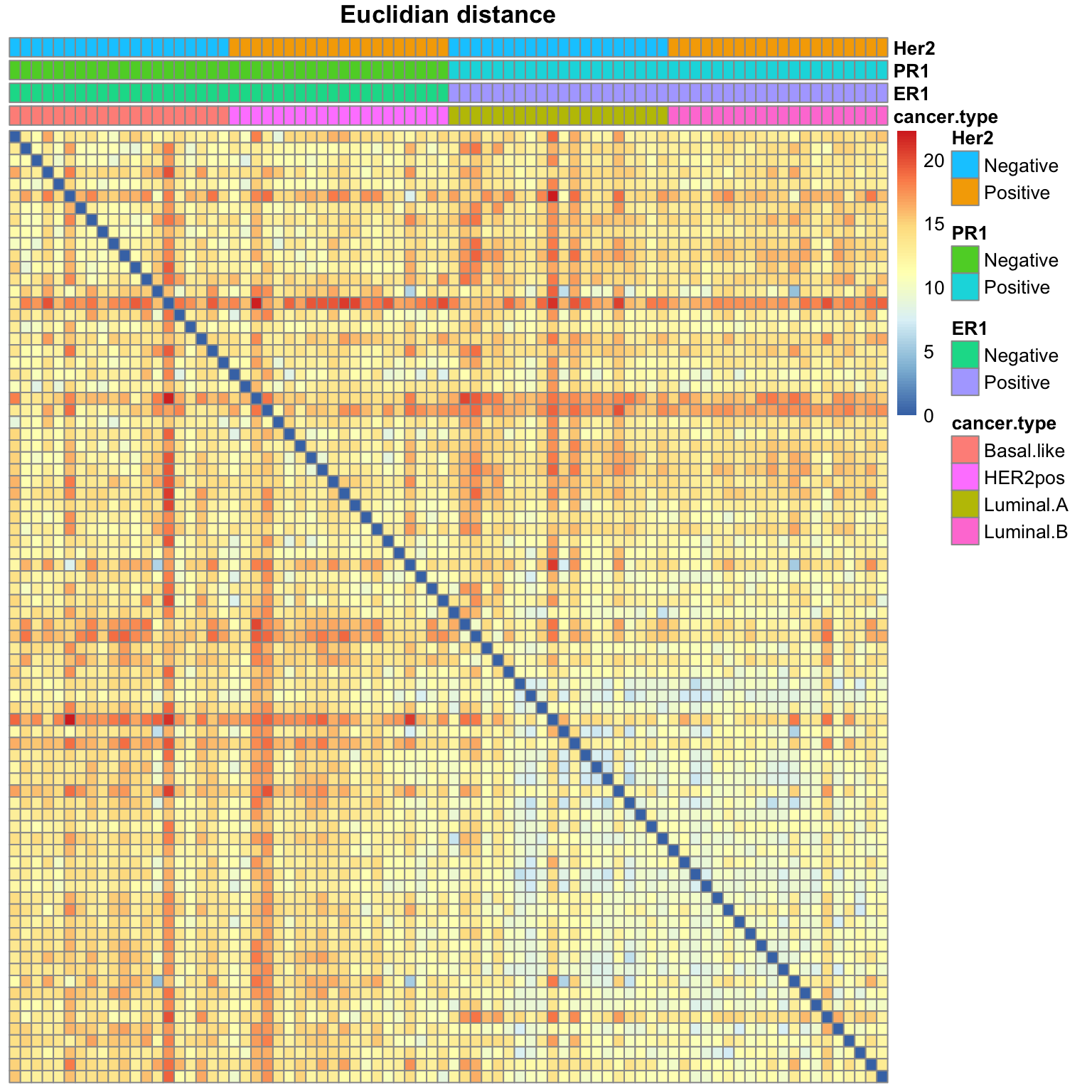
Heatmap of the Euclidian distance
Exercise: distance heatmaps
Run the same analysis for the Pearson and Spearman distance matrices. Interpret the results: do some of these measures seem more relevant to highlight the similarities between samples?
#### Pearson distance heatmap ######## Spearman distance heatmap ####Interpretation: dissimilarity measures
Comparing the three distance heatmaps above, can you already conclude something about the most relevant measure of dissimilarity between samples?
- TO BE COMPLETED
Computing a tree from a distance matrix
Use the function hclust() to get trees from the previously computed distance matrices.
Example: Euclidian matrix, complete linkage
#### Sample tree with Euclidian distance, complete linkage ####
sample_tree_euclidian_complete <- hclust(
  d = sample_dist_euclidian, method = "complete")

plot(sample_tree_euclidian_complete,
     xlab = NA, ylab = NA, hang = -1)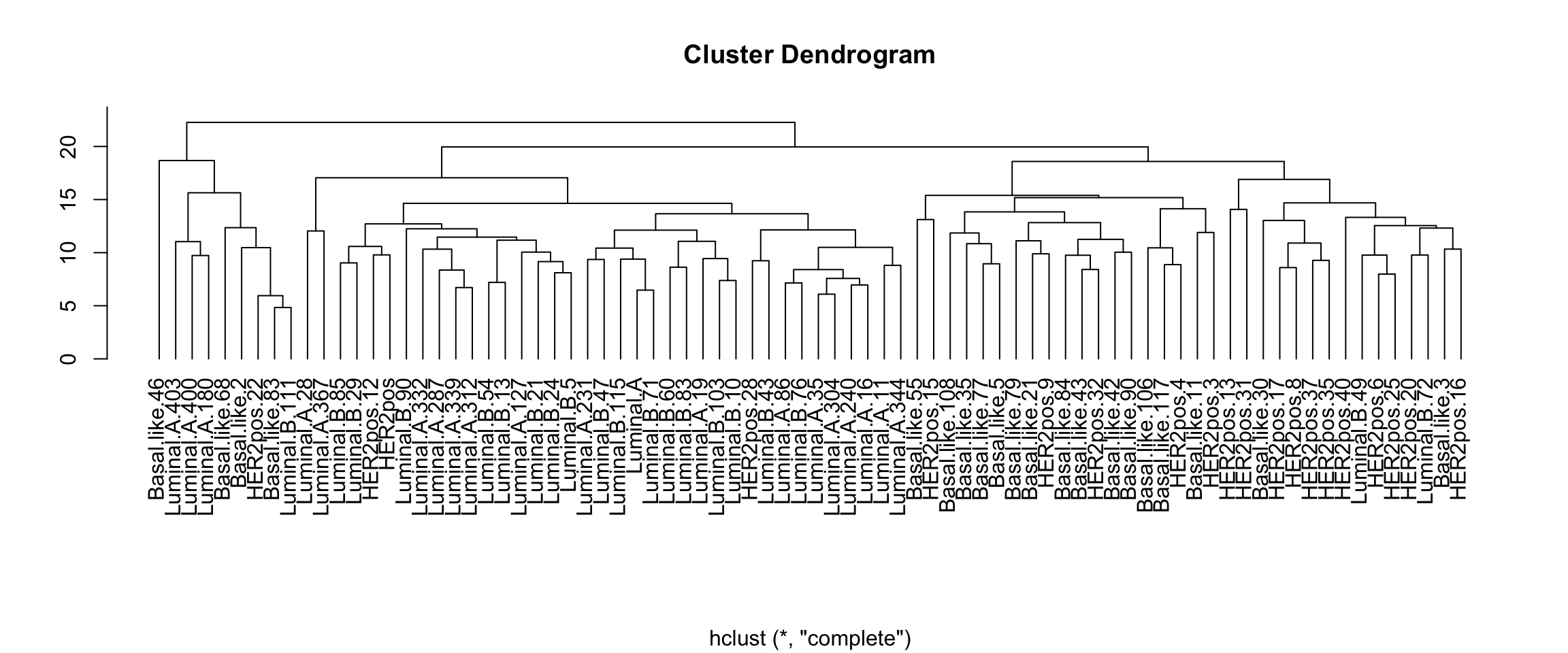
Sample tree of the expression matrix with Euclidian distance and complete linkage.
We can also use some fancy library (e.g. ClassDiscovery) to color the tree labels. Other librairies can be used to generate nice tree drawings, don’t hesitate to google and improve.
library(ClassDiscovery)
ClassDiscovery::plotColoredClusters(
  sample_tree_euclidian_complete,
  labs = subset_meta$cancer.type, ## class labels
  col = "grey", ## tree color
  cols = subset_meta$color,
  cex = 0.6,
  main = "Euclidian distance, Ward linkage")

legend("topright",
       legend = names(class_color),
       col = class_color,
       text.col = class_color, cex=0.9)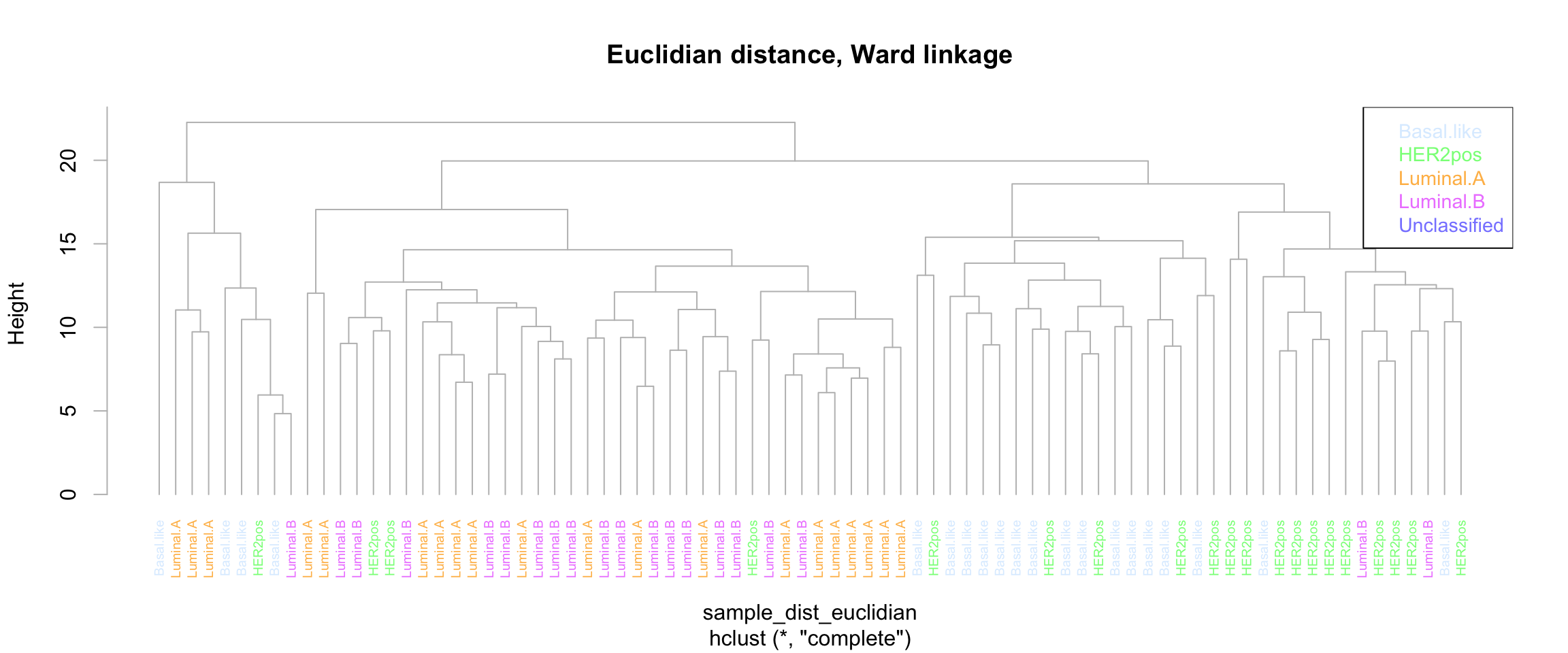
Sample tree of the expression matrix with Euclidian distance and complete linkage.
Exercises: other matrices and linkage rules
Test the different agglomeration rules (single, average, complete, ward) and the different disimilarity measures (Euclidian, Spearman, Pearson).
Interpretation: agglomeration rule
Based on the analyses above, would you consider that some agglomeration rules are generally more relevant than other ones with this dataset? If so, is it systematic or does the best agglomeration rule vary depending on the dissimilarity measure?
Tree cut
Cut the tree to obtain 4 samples clusters from the tree obtained with Euclidian distance and complete linkage.
Create a confusion matrix to compare the sample compositon of the clusters with the cancer types annotated in the metadata.
Compute the ARI from this confusion matrix.
#### Cluster - cancer type comparison ####

## Cut the tree
nclust <- 4
clusters_euclidian_complete <- cutree(
  tree = sample_tree_euclidian_complete, k = nclust)
confusion_euclidian_complete <- table(
  clusters_euclidian_complete,
  subset_meta$cancer.type)

kable(confusion_euclidian_complete, row.names = TRUE)| Basal.like | HER2pos | Luminal.A | Luminal.B | |
|---|---|---|---|---|
| 1 | 16 | 16 | 0 | 2 |
| 2 | 3 | 1 | 3 | 1 |
| 3 | 1 | 0 | 0 | 0 |
| 4 | 0 | 3 | 17 | 17 |
## Compute Adjusted Rand Index (ARI)
ari_euclidian_complete <- round(
  digits = 3,
  aricode::ARI(
    c1 = clusters_euclidian_complete,
    c2 = subset_meta$cancer.type))

message("ARI for Euclidian distance and complete linkage: ",
        ari_euclidian_complete)
With Euclidian distance and the complete lin,kage, we obtain an Adjusted Rank Index (ARI) of 0.312, computed with a subset of the expression table.
The next question is of course: can we obtain better results with other distances and agglomeration rules? This will be left as an exercise.
Clustering with the full dataset
Compute the ARI index with the same similarity measure and the same agglomeration rule, but with the full dataset (bic_expr_labels)
## Choose the clustering parameters
distance <- "euclidian"
rule <- "complete"

message("Computing ARI with ",
        distance, " dissimilarity and ",
        rule, " linkage")

## Euclidian distance
bic_dist <- factoextra::get_dist(
  x = t(bic_expr_labels), method = distance)

#### Sample tree with Euclidian distance, complete linkage ####
sample_tree <- hclust(
  d = bic_dist, method = rule)

## Confusion matrix
nclust <- 4
bic_clusters <- cutree(
  tree = sample_tree, k = nclust)
bic_confusion <- table(
  bic_clusters,
  bic_meta$cancer.type)

kable(bic_confusion, row.names = TRUE,
      caption = paste0(
        "Confusion table of the sample clusters versus cancer subtypes (all samples and 1000 genes). ",
        "Distance: ", distance, ". ",
        "Agglomeration rule: ", rule, ". "

))| Basal.like | HER2pos | Luminal.A | Luminal.B | Unclassified | |
|---|---|---|---|---|---|
| 1 | 117 | 40 | 378 | 106 | 100 |
| 2 | 4 | 0 | 0 | 0 | 3 |
| 3 | 9 | 1 | 18 | 7 | 4 |
| 4 | 1 | 0 | 26 | 5 | 0 |
## Compute Adjusted Rand Index (ARI)
bic_ari <- round(
  digits = 3,
  aricode::ARI(
    c1 = bic_clusters,
    c2 = bic_meta$cancer.type))

message("ARI for Euclidian distance and complete linkage (full dataset): ",
        bic_ari)
With Euclidian distance and the complete lin,kage, we obtain an Adjusted Rank Index (ARI) of -0.011, computed with a subset of the expression table.
Heatmap with biclustering (samples + genes)
Biclustering amounts to cluster both the individuals (patient samples in our case) and variables (genes in our case).
We will illustrate this with the Spearman correlation as distance and Ward as agglomeration rule.
#### Biclustering ####

# left as an exercise
Personal work: chosing the most relevant parameters
These analyses can be led collectively: each trainee could take one combination of parameters.
Based on the examples above, find the most relevant parameters (dissimilarity matrix, agglomeration rule) to cluster the samples of the subset expression matrix. Choose these parameters based on the confusion matrix and the ARI.
Draw different graphical representations of the best result:
- heatmap of the distance matrix
- sample tree with coloring of the annotated cancer type
- heatmap (samples x genes) with coloring of the metadata
Use these optimal parameters to run clustering with all the samples of the BIC dataset and the `1000 genes instead of the subset of 100. Export a table with the sample clusters and another one with the gene clusters.
Session info
As usual, we write the session info in the report for the sake of traceability.
sessionInfo()R version 4.0.2 (2020-06-22)
Platform: x86_64-apple-darwin17.0 (64-bit)
Running under: macOS Mojave 10.14.6
Matrix products: default
BLAS: /Library/Frameworks/R.framework/Versions/4.0/Resources/lib/libRblas.dylib
LAPACK: /Library/Frameworks/R.framework/Versions/4.0/Resources/lib/libRlapack.dylib
locale:
[1] en_US.UTF-8/en_US.UTF-8/en_US.UTF-8/C/en_US.UTF-8/en_US.UTF-8
attached base packages:
[1] stats graphics grDevices utils datasets methods base
other attached packages:
[1] ClassDiscovery_3.3.13 oompaBase_3.2.9 cluster_2.1.1 scales_1.1.1 pheatmap_1.0.12 aricode_1.0.0 factoextra_1.0.7 ggplot2_3.3.3 knitr_1.31
loaded via a namespace (and not attached):
[1] Rcpp_1.0.6 oompaData_3.1.1 highr_0.8 RColorBrewer_1.1-2 bslib_0.2.4 compiler_4.0.2 pillar_1.5.1 jquerylib_0.1.3 tools_4.0.2 mclust_5.4.7 digest_0.6.27 lattice_0.20-41 jsonlite_1.7.2 evaluate_0.14 lifecycle_1.0.0
[16] tibble_3.1.0 gtable_0.3.0 pkgconfig_2.0.3 rlang_0.4.10 Matrix_1.3-2 DBI_1.1.1 ggrepel_0.9.1 yaml_2.2.1 xfun_0.22 withr_2.4.1 stringr_1.4.0 dplyr_1.0.5 generics_0.1.0 sass_0.3.1 vctrs_0.3.6
[31] grid_4.0.2 tidyselect_1.1.0 glue_1.4.2 R6_2.5.0 fansi_0.4.2 rmarkdown_2.7 farver_2.1.0 purrr_0.3.4 magrittr_2.0.1 ellipsis_0.3.1 htmltools_0.5.1.1 assertthat_0.2.1 colorspace_2.0-0 utf8_1.2.1 stringi_1.5.3
[46] munsell_0.5.0 crayon_1.4.1